Substitution – Yes or No?

Substitution Thumbnail
Mathieu Westerweele
Mathieu Westerweele
Posted on:
29 Sep 2013
It is often seen that model designers insist on eliminating the extensive variables from their model equations. The main reason that is brought up for this preference to write a model that does not involve the extensive variables is that often only the evolution of the application variables (e.g. intensive or geometrical variables) is of interest.
Also, the transfer laws and kinetic laws are usually given in terms of intensive state variables. Therefore most model designers think they must transform the accumulation terms of the (differential) balance equations and perform a so-called state variable transformation.
In most textbooks that cover modelling these transformations are also performed, often even without mentioning why. But are these, often cumbersome, state variable transformations necessary to solve the considered problems?
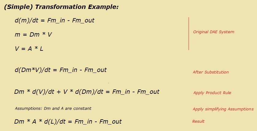
Above you see a simple example transformation that is often used, when someone would be interested in the dynamic response of the level of a tank.
An even more common transformation (which most model designers often do not even realise!), is the transformation of an Energy Balance (via the Enthalpy Balance) into an equation that represents the dynamic response of the Temperature of a system.
So, usually a modified version of this basic energy balance is employed for modelling a process component. This modified version is derived from the basic energy balance through several simplifications and assumptions.
Caution should be taken, though, when you use derived energy models, because they are often incorrect or used incorrectly. You could easily introduce faults when you are adapting or further simplifying a derived model, because of lack of knowledge about previous assumptions and derivation steps. Knowledge about the common assumptions and the derivation steps is thus essential for the correct use of the different simplified energy models.
In most cases, the transformations are not necessary. There are several reasons to consider the differential algebraic equations (DAEs) directly, rather than to try to rewrite them as a set of ordinary differential equations (ODEs):
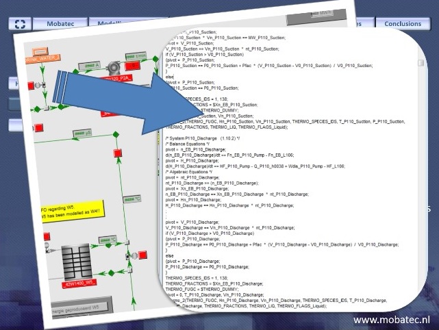
First, when modelling physical processes, the model takes the form of a DAE, depicting a collection of relationships between variables of interest and some of their derivatives. These relationships may be generated by a modelling program (such as Mobatec Modeller). In that case, or in the case of highly nonlinear models, it may be time consuming or even impossible to obtain an explicit model.
Computational causality is, quite obviously, not a physical phenomenon, but a numerical artefact. Take, for example, the ideal gas law:

pV = nRT


This is a static relation, which holds for any ideal gas. This equation does not describe a cause-and-effect relation. The law is completely impartial with respect to the question whether at constant temperature and constant molar mass a rise in pressure causes the volume of the gas to decrease or whether a decrease in volume causes the pressure to rise. For a solving program, however, it does matter whether the volume or the pressure is calculated from this equation.
It is rather inconvenient that a model designer must determine the correct computational causality of all the algebraic equations that belong to each modelling object, given a particular use of the model (simulation, design, etc.). It is much easier if the equations could just be described in terms of their physical relevance and that a computer program automatically determines the desired causality of each equation and solves each of the equations for the desired variable (either numerically or by means of symbolic manipulation).
Also, reformulation of the model equations tends to reduce the expressiveness.
Furthermore, if the original DAE can be solved directly it becomes easier to interface modelling software directly with design software.
Finally, reformulation slows down the development of complex process models, since it must be repeated each time the model is altered, and therefore it is easier to solve the DAE directly.
These advantages enable researchers to focus their attention on the physical problem of interest. There are also numerical reasons for considering DAEs. The change to explicit form, even if possible, can destroy sparsity and prevent the exploitation of system structure.
Small advantages of transforming the model to ODE form can be that for (very) small systems an analytical solution is available and that sometimes less information of physical properties is needed when substitutions are being made (sometimes, some of the parameters can be removed from the system equations when substitutions are made).
Another advantage could be that, by doing substitutions, some primary state variables are removed from the model description which could take the code faster, because less variables have to be solved.
In general, though, these advantages do not outweigh the disadvantages.
If one does want to perform substitutions, it is recommended that these are done at the very end of the model development and not, as is generally seen, as soon as possible. Postponing the substitutions as long as possible gives a much better insight in the model structure during model development.
I am very interested in your view on this subject:
Are you using substitutions in your dynamic models? Were you aware of the assumptions that are made by applying substitutions?
I invite to post your comments, insights and/or suggestions in the comment box below.
To your success!
Mathieu.

Is “Serious Gaming” useful in Chemical Engineering?

 Thumbnail
Mathieu Westerweele
Mathieu Westerweele
Posted on:
30 Aug 2013
According to the definition on Wikipedia “Serious Games are simulations of real-world events or processes designed for the purpose of solving a problem.
According to the definition on WikipediaSerious Games are simulations of real-world events or processes designed for the purpose of solving a problem. Although serious games can be entertaining, their main purpose is to train or educate users, though it may have other purposes, such as marketing or advertisement. Serious game will sometimes deliberately sacrifice fun and entertainment in order to achieve a desired progress by the player. Serious games are not a game genre but a category of games with different purposes. This category includes some educational games and advergames, political games, or evangelical games. Serious games are primarily focused on an audience outside of primary or secondary education.
In this month’s blog I would like to start a discussion about the usefulness of Serious Games within Chemical Engineering education and in the Process Industry.
In my opinion, one of the best ways for a new operator to learn the ins and outs of a plant he started working with, is to let him solve all kinds of real problems or situations that can occur during operation of the plant. Since a real plant normally runs very stable for long periods of time, it’s not very convenient to let an operator “play” with the real plant. A very good alternative would be to have a high-fidelity Operator Training Simulator to learn the process.
Operator Training Simulators can be seen as a first generation of Serious Games for chemical engineers and have already been around for decades. They started out as hardware-based solutions, but in the 1980s OTS applications became available for PCs. In the last decade a new innovation became available: A virtual reality component showing the outside operator view. This 3D world is dynamically linked to the process simulator.
OTS Screenshot
Screenshot of an OTS screen of more than 20 years ago..
With a 3D visualization a “Virtual Outside Operator” can actually open and close hand-operated valves, start and stop pumps, take field reading, see and hear equipment running, communicate with the control room, etc.. Instructors can mentor and manage training sessions, instead of being tied up in role playing the functions of an Outside Operator of previously provided “remote function” switches.
At Mobatec we also have several years of experience of linking (real-time) dynamic process models to 3D visual plants. The 3D graphics are developed for us by the high-tech company ExplainMedia. Have a look at the short video if you are not sure what a 3D visualization of a plant is. I regularly show interactive examples of these very attractive and intuitive, dynamic 3D modules to lecturers at Chemical Engineering departments or technical staff of a chemical plant and initially they react very enthusiastically. However, when talking a bit longer to get a feel for if they would be interested in having such a 3D module from their own environment, they usually become more reluctant.
A feedback I often get when talking to these people is that adding a 3D world to the education or training modules would be a “nice to have”, but not a “must”. Which, of course, typically translates to “we would really like to have it, but it must be cheap!”. However, realizing a cheaper solution for industry, especially when looking at education, would also imply/ have as a side-effect that a lot Universities and Schools should be potentially interested in 3D modules. Otherwise it would not be worth the investment.
I am very interested in your view on this subject:
Are interactive 3D visualizations of (parts of) chemical processes a valuable addition to a Chemical Engineering education and/ or learning tools of processing plants?
I invite to post your comments, insights and/or suggestions in the comment box below.
To your success!
Mathieu.
———————————————–

Structurally Consistent Dynamic Process Models

Consistent Dynamic Process Models Thumbnail
Mathieu Westerweele
Mathieu Westerweele
Posted on:
28 Jul 2013
In this month’s blog I will attempt to present a “roadmap” for constructing structurally consistent and solvable dynamic process models.
In this month’s blog I will attempt to present a “roadmap” for constructing structurally consistent and solvable dynamic process models. I tried to keep it short and simple, but I soon realised that this was nearly impossible, since leaving out certain details would make it difficult for a reader to grasp the complete picture.
So, this blog is a bit longer than usual. But if you take the time to consume it, you will certainly get more insight in how to properly set up a correct, structurally solvable dynamic process model (using any equation based solver).
A more thorough discussion on this subject is given in the document “Concepts and Modelling Methodology”. Just click on the link to download a copy.
 

Balance Equations

In order to characterize the behaviour of a process, information is needed about the natural state of this process (at a given time) and about the change of this state with time. The natural state of a process can be described by the values of a set of fundamental extensive quantities, while the change of state is given by the balance equations of those fundamental variables.
The fundamental extensive variables represent the ”extent” of the process c.q. the quantities being conserved in the process. In other words: they represent quantities for which the conservation principle and consequently also the superposition principle applies. So, for these variables, the balance equations are valid. In most chemical processes, the fundamental variables are: component mass, total energy and (sometimes) momentum.
The dynamic behaviour of a system can be modelled by applying the conservation principles to the fundamental extensive quantities of the system. The principle of conservation of any extensive quantity (x) of a system states that what gets transferred into the system must either leave again or is transformed into another extensive quantity or must accumulate in the system (In other words: no extensive quantity is lost).
In my PhD thesis I showed that the dynamic part (i.e. the differential equations) of physical-chemical-biological processes can be represented in a concise, abstract canonical form, which can be isolated from the static part (i.e. the algebraic equations). This canonical form, which is the smallest representation possible, incorporates very visibly the structure of the process model as it was defined by the person who modelled the process: The system decomposition (physical topology) and the species distribution (species topology) are very visible in the model definition. The transport (z) and production (r) rates always appear linearly in the balance equations, when presented in this form:

dx/dt = Az+ Br

in which:
  • x :: Fundamental state vector (Primary State vector)
  • z :: Flow of extensive quantities (Transport rates)
  • r :: Kinetics of extensive quantity conversion (Reaction rates)
  • A :: Interconnection matrix
  • B :: Stoichiometric coefficient matrix

  The classification of variables that is presented here is, in the first place, based on the structural elements of the modelling approach (namely systems and connections).
The matrices A and B are completely defined by the model designer’s definition of the physical and species topology of the process under investigation. Therefore these matrices are trivial to setup (and are actually automatically constructed by Mobatec Modeller). The only things a model designer has to do to complete the model are:
  • Provide a link between the transport and reaction rate vectors and the primary state vector. Each element in the transport and reaction rate vectors has to be (directly or indirectly) linked to the primary state vector. This “linking” is done with one or more algebraic equations. If certain elements of the rate vectors are not defined in the algebraic equations, the mathematical system will have too many unknowns and can consequently not be solved.
  • Give a mapping which maps the primary state of each system in a secondary state. This mapping is necessary because usually transport and reaction rates are defined as functions of secondary state variables (a heat flow can, for example, be expressed as a function of temperature difference).


Algebraic Equations

So, in addition to the balance equations, we need other relationships to express thermodynamic equilibria, reaction rates, transport rates for heat, mass, momentum, and so on. Such additional relationships are needed to complete the mathematical modelling of the process. A model designer should be allowed to choose a particular relationship from a set of alternatives and to connect the selected relationship to a balance equation or to another defined relationship. The algebraic equations are divided into three main classes, namely system equations, connection equations and reaction equations.
 

System Equations

For each system that is defined within the physical topology of a process, a mapping is needed which maps the primary state variables (x) into a set of “secondary state” variables (y = f(x)). The primary states of a system are fundamental quantities for describing the behaviour of the system. The fundamental state is defined intrinsically through the fundamental behaviour equations. The application of fundamental equations of component mass and energy balances intrinsically defines component mass and energy as the fundamental state variables. Alternative state variables are required for the determination of the transfer rate of extensive quantities and their production/consumption rate.
The equations that define secondary state variables do not have to be written in explicit form, by the way, but it has to be possible to solve the equations (either algebraically or numerically) such that the primary state can be mapped into the secondary state. This means that each defined equation has to define a new variable. Equations that link previously defined variables together are not allowed, since the number of equation would then exceed the number of variables and the set of equations of this system would thus be over-determined.
 

Connection Equations

The flow rates (z), which emerge in the balance equations of a system, represent the transfer of extensive quantities to and from adjacent systems. These flow rates can be specified or linked to transfer laws, which are usually empirical or semi-empirical relationships. These relationships are usually functions of the states, and the physical and geometrical properties of the two connected systems. For example, the rate of conductive heat transfer Q through a surface A between two objects with different temperatures can be given by:

Q = U * A *(Tor-Ttar)

This relationship depends on the temperatures Tor and Ttar of the origin and target object respectively. Temperature is of course a (secondary) state variable. The rate of heat transfer also depends on the overall heat transfer coefficient U, which is a physical property of the common boundary segment between the two systems, and on the total area of heat transfer A, which is a geometrical property.
A transfer law thus describes the transfer of an extensive quantity between two adjacent systems (z = f(yor, ytar)). The transfer rate usually depends on the state of the two connected systems and the properties of the boundary in between.
 

Reaction Equations

Depending on the time scale of interest, we can divide reactions into three groups:
  • Very slow reactions (slow in the measure of the considered range of time scales). These reactions do not appreciably occur and may be simply ignored.
  • Reactions that occur in the time-scale of interest. For these reactions kinetic rate laws can be used.
  • Very fast reactions (relative to the considered time scale), for which is assumed that the equilibrium is reached instantaneously.

  As the non-reactive parts do not further contribute to the discussion, they are left out in the sequel. The fast (equilibrium) reactions go beyond the scope of this blog and are therefore also not discussed.
For the “normal” reactions the reaction rates of the reactions in the relevant times scale must be defined by kinetic rate equations. The production terms are linked to kinetic laws, which are empirical equations. They are usually written as a function of a set of intensive quantities, such as concentrations, temperature and pressure (r = f(ysys)). For example, the reaction rate r of a first-order reaction taking place in a lump is given by:

r = V * k0 * exp(-E/(R * T))*ca

where:
  • r :: Reaction rate of a first-order reaction
  • V :: Volume of the system
  • k0 :: Pre-exponential kinetic constant
  • E :: Activation energy for the reaction
  • R :: Ideal gas constant
  • T :: Temperature of the reacting system
  • Ca :: Concentration of component A in the system

  Temperature and concentration(s) of the reactive component(s) are state variables (y) of the reactive system. Reaction constants and their associated parameter such as activation energy and pre-exponential factors are physical properties. In some cases, also geometrical properties of the system are part of the definition of the kinetic law, such as the porosity or other surface characterizing quantities.

Consclusions

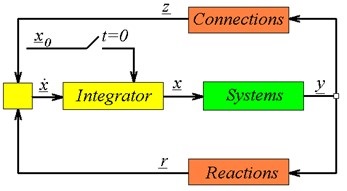
When a dynamic process model is formulated and proper initial conditions have been defined, then the information flow of a simulation can be depicted as in the above figure. Starting from the initial conditions x0, the secondary state variables y of all the systems can be calculated (via the System Equations y=f(x)). Subsequently, the flow rates z of all the defined connections and the reaction rates r of all the defined reactions can be calculated (z = f(yor, ytar); r = f(ysys)). These rates are the inputs of the balance equations, so now the integrator can compute values for the primary state variables x on the next time step. With these variables, the secondary state y can be calculated again and the loop continues until the defined end time is reached.
To put it in other words: A model designer should only be concerned with the algebraic equations (the right hand side of the figure), which means that the primary state variables x of each system can be considered as “known”. Systems are only interacting with each other through connections and therefore the calculation of the secondary variables of each system can be done completely independent of other systems.
The system equations map the primary state x into a secondary state y for each individual system, and each defined equation has to define a (secondary) variable. In some cases two or more equations may introduce two or more new variables, such that these equations have to be solved simultaneously in order to get a value for the variables.
For connection and reaction equations a similar conclusion can be drawn. For these equations the secondary variables of the systems (y) can be considered as “known”.
Looking at modelling like this, makes it a lot easier than trying to understand/debug the complete model of a process. Just divide your model into systems and connections, assign equations to those objects (typically not more than 10) and solve any problem that arises per object. Resolving a problem (or even several) of about 10 equations is a lot easier than when hundreds or more are considered at the same time!
Do you have experience with making (large) dynamic process models?
I invite to post your experiences, insights and/or suggestions in the comment box below, such that we can all learn something from it.
To your success! Mathieu.
———————————————–

A closer look at process model equations

Closer Look at Process Model Equations Thumbnail
Mathieu Westerweele
Mathieu Westerweele
Posted on:
28 Jun 2013
I couldn’t agree more with the statement that modelling is far more than just writing equations; the modelling activity should not be considered separately but as an integrated part of a problem solving activity. But, as promised in the previous blog, I would like to spend some lines on setting up equations for your process model.
“Process modelling is one of the key activities in process systems engineering… In most books on this subject there is a lack of a consistent modelling approach applicable to process systems engineering as well as a recognition that modelling is not just about producing a set of equations. There is far more to process modelling than writing equations”. These are a few lines from the introduction of the book “Process Modelling and Model Analysis” of Katalin Hangos and Ian Cameron. It is one of the best books around on the subject and it gives a comprehensive treatment of process modelling useful to students, researchers and industrial practitioners.
I couldn’t agree more with the statement that modelling is far more than just writing equations; the modelling activity should not be considered separately but as an integrated part of a problem solving activity. But, as promised in the previous blog, I would like to spend some lines on setting up equations for your process model.
Before we start, it is good to repeat that modelling a chemical process requires the use of all the basic principles of chemical engineering science, such as thermodynamics, kinetics, transport phenomena, etc. It should therefore be approached with care and thoughtfulness.
A (mathematical) model of a process is usually a system of mathematical equations, whose solutions reflect certain quantitative aspects (dynamic or static behaviour) of the process to be modelled. The development of such a mathematical process model is initiated by mapping a process into a mathematical object. The main objective of a mathematical model is to describe some behavioural aspects of the process under investigation.
There are many ways to generate these equations and there are many different ways to describe the same process, which will usually result in different models. The approach a modeller takes when constructing a model for a process depends on:
  • The application for which the model is to be used. Different models are used for different purposes. For example, a model which is used for the control of a process shall be different from a model which is used for the design or analysis of that same process
     
  • The amount of accuracy that has to be employed. This is of course partially depending on the application of the model and on the time-scale in which the process has to be modelled. In general, a model which needs to describe a process on a small time-scale demands more details and accuracy then the model of the same process which describes the process over a larger time-scale;
     
  • The view and knowledge of the modeller on the process. Different people have different backgrounds and different knowledge and will therefore often approach the same problem in different ways, which can eventually lead to different models of the same process.
     
The construction of the physical topology and species topology of a process are rather straight forward. When introducing the equations into the model, we are faced with some non-trivialities that need some closer look.
Having completed the first two stages of the modelling process, it is quite trivial to construct the dynamic part of the process model, namely the (component) mass and energy balances for all the systems, using the conservation principles. The resulting (differential) equations consist of flow rates and production rates, which should not be further specified at this point.
In order to fully describe the behaviour of the process, all the necessary remaining information (i.e. the mechanistic details) has to be added to the symbolic model of the process. So, in addition to the balance equations, other relationships (i.e. algebraic equations) are needed to express transport rates for mass, heat and momentum, reaction rates, thermodynamic equilibrium, and so on. The resulting set of differential and algebraic equations (DAEs) is called the equation topology.
From a certain point of view the modelling process can thus be regarded as a succession of equation-picking and equation-manipulation operations. The modeller has, virtually at least, a knowledge base containing parameterized equations that may be chosen at certain stages in the modelling process, appropriately actualized and included in the model. The knowledge base is, in most cases, simply the physical knowledge of the modeller, or might be a reflection of some of his beliefs about the behaviour of the physical process.
The equation topology forms a very important part of the modelling process, for with the information of this topology the complete model of the process is generated. The objective of the equation topology is the generation of a mathematically consistent representation of the process under the view of the model designer (who mainly judges the relative dynamics of the various parts, thus fixes intrinsically the dynamic window to which the model applies)
Information Flow
 
I realise that I’m just scratching the surface here, but a thorough discussion would be quite lengthy and probably just for a small audience. In the next blog I will, however, go into detail a bit more and will try to convey to you that once you understand the picture just above this text, you actually understand how any dynamic process model should be setup in order to be structurally solvable.
For now it will remain a bit abstract, but it gives you something to think about in the coming weeks :).
If you think you know what the picture represents, let everybody know by placing a comment in the comment box below. Any other comments, suggestions or questions regarding the topic of this blog would, of course, also be greatly appreciated.
To your success! Mathieu.
———————————————–

Assistance in Setting Up Models

Setting up models Thumbnail
Mathieu Westerweele
Mathieu Westerweele
Posted on:
28 May 2013
More often than not, the time spent on collecting the information necessary to properly define an adequate model of the (part of the) process you are interested in is much greater than the time spent by a simulator program in finding a solution.
More often than not, the time spent on collecting the information necessary to properly define an adequate model of the (part of the) process you are interested in is much greater than the time spent by a simulator program in finding a solution. Most publications and textbooks present the model equations without a description of how the model equations have been developed. Hence, to learn dynamic model development, novice modellers must study examples in textbooks, the work of more skilled modellers, and/or use trial and error.
During the last decades there tends to be an increasing demand for models of higher complexity, which makes the model construction even more time consuming and error-prone. Moreover, there are many different ways to model a process (mostly depending on the application for which the model is to be used): different time scales, different levels of detail, different assumptions, different interpretations of (different parts of) the process, etc. Thus a vast number of different models can be generated for the same process.
All this calls for a systematisation of the modelling process, comprising of an appropriate, well-structured modelling methodology for the efficient development of adequate, sound and consistent process models. A Modelling tool building on such a systematic approach supports teamwork, re-use of models, provides complete and consistent documentation and, not at least, improves process understanding and provides a foundation for the education of process technology.
As promised in our last blog post, this months blog presents some of the concepts of Mobatec Modeller, a computer-aided modelling tool built on a structured modelling methodology, which aims to effectively assist in the development of process models and helps and directs a modeller through the different steps of this methodology. The objective of this tool is to provide a systematic model design method that meets all the mentioned requirements and turns the art of modelling into the science of model design.
Modelling is an acquired skill, and the average user finds it difficult. A modeller may inadvertently incorporate modelling errors during the mathematical formulation of a physical phenomenon. Formulation errors, algebraic manipulation errors, writing and typographical errors are very common when a model is being implemented in a computing environment. Thus any procedure which would allow to do some of the needed modelling operations automatically would eliminate a lot of simple, low-level (and hard to detect) errors.
Mobatec Modeller is a computer-aided modelling tool which is designed to assist a model designer to map a process into a mathematical model, using a systematic modelling methodology. The main task solved by Mobatec Modeller is the construction and manipulation of the structure and definition of process models. The output of Mobatec Modeller is a first-principles based (i.e. based on physical insight) mathematical model, which is easily transformed to serve as an input to existing modelling languages and/or simulation packages, such as our Mobatec Solver, but also Process Studio’s e-Modeler (Protomation), gProms (Process Systems Enterprise), Aspen Custom Modeler (Aspentech), Modelica (Dynasim AB), Matlab (Mathworks), or any other Differtial Algebraic Equation (DAE) Solver. For certain solvers (Mobatec Solver and e-Modeler) a Simulation Environment is available, such that the build dynamic process models can be excecuted, tuned, tested, optimised, etc.
One of the handy features of Mobatec Modeller that will help a model designer a lot when setting his process model is the Automatic component distribution.
 

Automatic component distribution

The distribution of all involved species (i.e. chemical and/or biological components) as well as all reactions in the various parts of the process must be defined in most process models. This represents the Species Topology, which is superimposed on the physical topology and defines which species and what reactions are present in each part of the physical topology.
The definition of the species topology of a process is initialized by assigning sets of species (and/or reactions) to some systems. Species as well as reactions should be selected from corresponding databases. So, before the species topology can be defined, a species and a compatible reactions database must be defined. Such a database contains a list of species and a list of possible reactions between those species. A species and reactions database should, of course, be editable by the user in order to satisfy the specific needs of the user.
After the assignment of the injected species and injected reactions to a specific system, the modelling tool will (re)calculate (parts of) the species distribution. This means that the species will propagate into other systems through mass connections. Within the systems, the species may undergo reactions and generate ”new” species, which in turn may propagate further and initiate further reactions. This eventually results in a specific species distribution over the elementary systems, which is referred to as the species topology of the processing plant.
Species Distribution
To enhance the definition of the species topology, permeability and directionality are introduced as properties of mass connections. They constrain the mass exchange between systems by making the species transfer respectively selective or uni-directional.
The injection of a reaction into a system does not automatically imply that this reaction can ”happen” in that system and thus that the products of this reaction can be formed. If not all reactants of a reaction are available in a system, then this reaction cannot take place in this system. In such a case, the system will have an injected reaction but this reaction will not be “active”. So, the reaction will not take place in the system in this case. When the species distribution is changed and the reaction can take place again, it will automatically be ”activated”.
It should be noted that the presence of an ”activated” reaction in a system does not imply that this reaction has to happen in this system. It implies that this reaction may happen in this system, depending on the operating conditions in the system and the driving force for this reaction.
Whenever an operation is executed which modifies the current species distribution, a mechanism is activated which updates the species distribution over all elementary systems and connections of the affected mass domains.
After the definition of the Species Topology, Mobatec Modeller can automatically generate the dynamic part of the process model, namely the (component) mass and energy balances for all the elementary systems, using the conservation principles. The resulting (differential) equations consist of flow rates and production rates, which are not further specified at this point. In order to fully describe the behaviour of the process, all the necessary remaining information (i.e. the mechanistic details) has to be added to the symbolic model of the process. So, in addition to the balance equations, other relationships (i.e. algebraic equations) are needed to express transport rates for mass, heat and momentum, reaction rates, thermodynamic equilibrium, and so on. The resulting set of differential and algebraic equations (DAEs) is called the equation topology.
In the next blog we will explore how Mobatec Modeller helps you in setting up correct (algebraic) equations for each part of your model.
This blog and the next blog focus a bit on how our tools can help model designers in setting up their models. Normally our blog treats more generic topics, related to modelling, but several people asked me to devote one or more blogs to the differences between our solutions and other available software ;).
Please let us know if you found this information valuable or specify a topic you would like to see discussed on one of the next blogs.
To your success!
Mathieu.
———————————————–