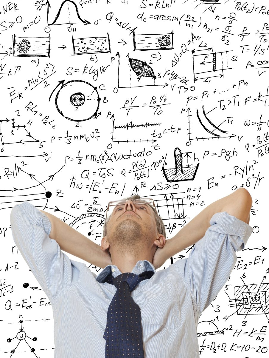
In our last blog post we discussed about fundamental time scale assumptions and the implication these assumptions can have on the final model. This month we discuss types of assumptions that have less effect on the structure and contents of the model, but that can certainly lead to (computational) problems if they are not recognized.
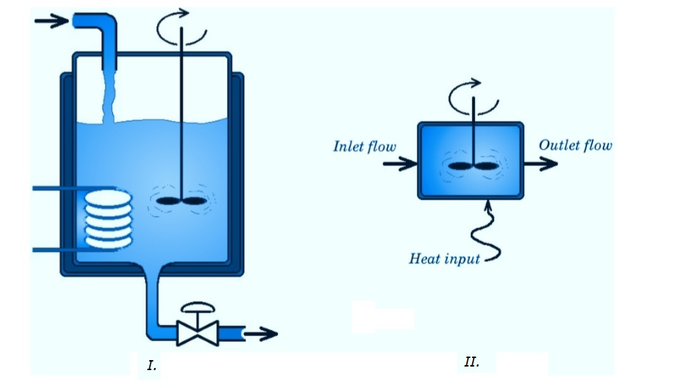
Constraints and assumptions describe all kinds of algebraic relationships between process quantities which have to hold at any time. A volume constraint, for example, restricts the volume of a simple system or the sum of volumes of a set of systems. Assumptions may result in models which are cumbersome to solve. Potential problems can very often be avoided at an early stage of the model development by keeping clear of certain assumptions or by directly dealing with the cause of the potential problems.
As discussed in the previous blog post one can distinguish between several types of assumptions: Structural assumptions (i.e. the construction of the physical topology), order of magnitude assumptions (very small versus very large) and assumptions on relative time scale (very slow versus very fast). These assumptions are usually introduced with a goal, namely to simplify the description of the behaviour by neglecting what is considered insignificant in the view of the application one has in mind for the model. Whilst indeed such assumptions do simplify the description, they are also the source of numerous problems, such as “index problems”, which make the solving of the equations very difficult.
 

High-index Models

Dynamic process models, as derived with our modelling methodology, consist of differential and algebraic equations (DAEs). Unfortunately, most engineers have little knowledge of the theory of DAEs, since most of the calculations that have to be performed during education are steady-state simulations. In the rare case that dynamics are considered, a mathematical description of the (usually very simple) model is derived in the form of ordinary differential equations (ODEs).
One of the major advantages of writing a model in DAE form as opposed to ODE form, is that a modeller does not have to perform a set of often cumbersome mathematical manipulations, such as substitution and symbolic differentiation. Dynamic process models can be divided into “low index” models (index 0 and 1) and “high index” models (index two and higher and some index one models). The differential index or index is a measure of the problems related to initialisation and integration of dynamic process models. The problems related to solve a dynamic process model increase with increasing index.
We will not go into details nor give a mathematically correct definition of the index of a model at this stage, but will just state that the index of a DAE is the number of times that all or part of a DAE must be differentiated (with respect to time) in order to get an ODE.
It is not recommend, by the way, to actually perform this series of differentiations as a general solution procedure for DAEs. Rather the number of such differentiation steps that would be required in theory turns out to be an important quantity in understanding the behaviour of numerical methods.
According to the definition an ODE (either explicit or implicit) has index zero. DAEs with index zero and one are generally much simpler to understand (and much simpler to solve) than DAEs with index two or higher.
With our modelling method we strive to produce semi-explicit index one models, since these can be easily used for simulation by any DAE-solver. Higher index models must either be simulated directly by a special integrator which tackles high index DAEs, or be transformed to semi-explicit index one and integrated. Two simple tests that guarantee structurally semi-explicit index one models are:

• All algebraic variables must be present in the algebraic equations.
• It must be possible to assign each algebraic equation to an algebraic variable. Assignment of all equations and variables must be possible.

If one or several algebraic variables are absent from the algebraic equations, then the model index is two or higher.
 

Assumptions Leading to High-index Models

Many high-index problems are caused by a model purpose that is not carefully considered, because the modeller does not want to include some of the rapid dynamics in the model, by assumptions that may not be essential or because the modeller wants to include certain variables in the model.
Our modelling method forces a model designer to be more aware of the assumptions he makes. Therefore, potential high index model formulations can be detected and/or avoided at an early stage of the model development. Knowing the causes of high index formulations helps the model designer in carefully considering the modelling purpose and the assumptions he wants to make.
Assumptions that impose direct or indirect constraints on the differential variables lead to high index models. But a modeller cannot simply impose some constraints on the differential variables. A constraint is always imposed by some “driving force” (i.e. a flow or reaction, since these are the only forces that appear in the differential equations), which forces the differential variables to adhere to the constraint. This means that instead of giving a description for the rate, a flow or reaction remains “unmodelled” and a (direct or indirect) constraint on the differential variables is given.
There can be several reasons why a modeller wants to introduce assumptions:

• Only slow dynamics of the process are of interest. In this case the rapid dynamics can be neglected.
• Difficulties in finding reliable rate equations may force a modeller to make quasi steady-state assumptions.
• In order to perform model reduction, simplifying assumptions may be introduced.

In our previous blog post the term time scale was introduced. Modelling systems in a range of time scales, the capacity terms are chosen accordingly but also the transport and the production terms. For parts being outside of the time scale in which the dynamics are being modelled, a pseudo steady-state assumption is made. For example, (very) fast reactions – fast in the measure of the considered range of time scale – are assumed to reach the equilibrium (for all practical purposes) instantaneously, and very slow ones do not appreciably occur and may be simply ignored.
In a next blog post we will zoom into “steady-state assumptions” and “events and discontinuities”.
What is your experience with constraints and assumptions? Did you ever run into computational problems without knowing what the cause was?
I invite to post your experiences, insights and/or suggestions in the comment box below, such that we can all learn something from it.
To your success!
Mathieu.
———————————————–

Physical topologies are the abstract representation of the containment of the process in the physical sense. They visualise the principle dynamic contents of the process model and therefore the construction of a physical topology is the most fundamental part of the modelling process. Any changes in the physical topology will substantially affect the structure and contents of the final model.
The structuring of the process implements the first set of assumptions in the modelling process. The resulting decomposition is, in general, not unique. However, the resulting model depends strongly on the choice of the decomposition. As a rule: the finer the decomposition, the more complex will the resulting model be.
The decision of defining subsystems is largely based on the phase argument, where the phase boundary separates two systems. The second decision criterion utilises the relative size of the capacities and the third argument is based on the relative velocity with which subsystems exchange extensive quantities. Another argument is the location of activities such as reactions. The relative size of the model components, measured in ratios of transfer resistance and capacities, termed time constants, is referred to as “granularity”. A large granularity describes a system cruder, which implies more simply, than a model with a finer granular structure. It seems apparent that one usually aims at a relative uniform granularity, as these systems are best balanced and thus more conveniently solved by numerical methods.
Models of different granularity help in analysing the behaviour of the process in different time scales. The finer the granularity, the more the dynamic details and thus the more of the faster effects are captured in the process description. Since each model is constructed for a specific goal, a process model should reflect the physical reality as accurately as needed. The accuracy of a model intended for numerical simulation, for example, should (in most cases) be higher than the accuracy of a model intended for control design.
To illustrate the concepts mentioned above, consider the following example concerning a stirred tank reactor: Figure I shows a stirred tank reactor, which consists of an inlet and outlet flow, a mixing element, a heating element and liquid contents. If the model of this tank is to be used for a rough approximation of the concentration of a specific component in the outlet flow or for the liquid-level control of the tank, a simple model suffices. The easiest way to model this tank is to view it as an ideally stirred tank reactor (ISTR) as shown in figure II. This implies that a number of assumptions have been made regarding the behaviour and properties of the tank. The most important assumption is the assumption that the contents of the tank is ideally mixed and hence displays uniform conditions over its volume. Another assumption can be that heat losses to the environment are negligible.
After making these and maybe some more assumptions, the modeller can write the component mass balances and the energy balance of the reactor. With these equations and some additional information (e.g. kinetics of reaction, physical properties of the contents, geometrical relations, state variable trans- formations, etc.) the modeller can describe the dynamic and/or static behaviour of the reactor. If the tank has to be described on a much smaller time-scale and/or the behaviour of the tank has to be described in more detail, then the ISTR model will not suffice. A more accurate description often asks for a more detailed model. In order to get a more detailed description the modeller could, for example, choose to try to describe the mixing process in the tank (see figure III). Figure IV shows a possible division of the contents of the tank into smaller parts. In this drawing a circle represents a volume element which consists of a phase with uniform conditions. Each volume element can thus be viewed as an ISTR. The arrows represent the mass flows from one volume to another. In order to describe the behaviour of the whole tank, the balances of the fundamental extensive quantities (component mass and energy usually suffice) must be established for each volume element. The set of these equations, supplemented with information on the extensive quantity transfer between the volumes and other additional information, will constitute the mathematical description of the dynamic and/or static behaviour of the reactor.
The model of the mixing process could, of course, be further extended to get a more accurate description. The number of volume elements could for example be increased or one could consider back mixing or cross mixing of the liquid between the various volume elements (In principle, if one increases the complexity of this description, one approaches the type of models that result from approximating distributed models using computational fluid dynamic packages). The conduction of heat to each volume could also be modelled. One could model a heat flow from a heating element to each volume, or only to those volume elements which are presumed to be the nearest to the heating element, etc. As one may imagine there are many ways to describe the same process. Each way usually results in a unique mathematical representation of the behaviour of the process, depending on the designers view on and knowledge of the process, on the amount of detail he wishes to employ in the description of the process and, of course, on the application of the model.
When employing the term time scale, we use it in the context of splitting the relative dynamics of a process or a signal (the result of a process) into three parts, namely a central interval where the process or signal shows a dynamic behaviour (1). This dynamic window is on one side guarded by the part of the process that is too slow to be considered in the dynamic description, thus is assumed constant (2). On the other side the dynamic window is attaching to the sub-processes that occur so fast that they are abstracted as event – they just occur in an instant (3). Any process we consider requires these assumptions and it is the choice of the dynamic window that determines largely the fidelity of the model in terms of imaging the process dynamics. One may argue that one should then simply make the dynamic window as large as probably possible to avoid any problems, which implies an increase in complexity. Philosophically all parts of the universe are coupled, but the ultimate model is not achievable. When modelling, a person must thus make choices and place focal points, both in space as well as in time. The purpose for which the model is being generated is thus always controlling the generation of the model. And the modeller, being the person establishing the model, is well advised to formulate the purpose for which the model is generated as explicit as possible.
A window in the time scales must thus be picked with the limits being zero and infinity. On the small time scale one will ultimately enter the zone where the granularity of matter and energy comes to bear, which limits the applicability of macroscopic system theory and at the large end, things get quite quickly infeasible as well, if one extends the scales by order of magnitudes. Whilst this may be discouraging, having to make a choice is usually not really imposing any serious constraints, at least not on the large scale. Modelling the movement of tectonic plates or the material exchange in rocks asks certainly for a different time scale than modelling an explosion, for example. There are cases, where one touches the limits of the lower scale, that is, when the particulate nature of matter becomes apparent. In most cases, however, a model is used for a range of applications that usually also dene the relevant time-scale window.
The dynamics of the process is excited either by external effects, which in general are constraint to a particular time-scale window or by internal dynamics resulting from an initial imbalance or internal transposition of extensive quantity. Again, these dynamics are usually also constraint to a time-scale window. The maximum dynamic window is thus the extremes of the two kinds of windows, that is, the external dynamics and the internal dynamics.
A “good” or “balanced” model is in balance with its own time scales and the time-scale within which its environment operates. In a balanced model, the scales are adjusted to match the dynamics of the individual parts of the process model. Balancing starts with analysing the dynamics of the excitations acting on the process and the decision on what aspects of the process dynamics are of relevance for the conceived application of the model. What has been defined as a system (capacity) before may be converted into a connection later and vice versa as part of the balancing process. This makes it difficult, not to say impossible, to define systems and connections totally hard. The situation clearly calls for a compromise, which, in turn, opens the door for suggesting alternative compromises. There is not a single correct choice and there is certainly room for arguments but also for confusion. Nevertheless a decision must be taken.
Initially one is tempted to classify systems based on their unique property of representing capacitive behaviour of volumes, usually also implying mass. In a second step one may allow for an abstraction of volumes to surfaces, because in some applications it is convenient to also abstract the length scale describing accumulation to occur inside, so-to-speak, or on each side of the surface.
What is your experience with time scale assumptions? Where you aware that you actually always make them, when modelling? Are you aware of the effect they have on your end results?
I invite to post your experiences, insights and/or suggestions in the comment box below, such that we can all learn something from it.
To your success!
Mathieu.
———————————————–

In the blog post of last month we discussed about the substitution of variables and whether these variable transformation are actually necessary to solve the problems at hand. Part of the discussion was concerned with the computational causality of the involved equations and this month I would like to spend a few more words on that topic.
As discussed in previous blog posts, the dynamic part (i.e. the differential equations) of a process model can be isolated from the static part (i.e. the algebraic equations). The dynamic part can be trivially derived from the model designer’s definition of the Physical Topology and Species Topology of the process. The static part has to be defined by the physical insight of the model designer.
For each modelling object (i.e. system, connection or reaction) the algebraic equations can, in principle, be chosen “randomly” from a database. In doing so, the problem arises that not every numerical equation solver will be able to solve the equations, since the equations are not in the so-called correct computational order and are not always in (correct) explicit form. Nowadays, many solvers (so-called DAE-1 solvers) can easily handle implicit algebraic equations, but when the equations are re-ordered and simplified by performing preliminary symbolic manipulations, a more efficient computational code could be obtained.
If you are using an explicit solver (such as Matlab) to solve your model equations, an important step to achieve an efficient computational code for DAEs, is to solve the equations for as many algebraic variables as possible. This way it is not necessary to introduce these variables as unknowns in the numerical DAE-solver, since they can be calculated at any call of the residual routine from the information available.
Consider the simple pair of equations:

y – 2x = 4  (1)

x – 7 = 0    (2)

In order to solve these equations directly, they must be rearranged into the form:

x = 7          (3)

y = 2x + 4  (4)

The implicit equation (2) cannot readily be solved for x by a numerical program, whilst the explicit form, namely (3), is easily solved for and only requires the evaluation of the right-hand-side expression. Equation (1) is rearranged to give (4) for y, so that when x is known, y can be calculated.
The rearranged form of the set of equations can be solved directly because it has the correct computational causality. As discussed in the blog on substitution, this computational causality is, quite obviously, not a physical phenomenon, but a numerical artefact. Take, for example, the ideal gas law:

pV = nRT

This is a static relation, which holds for any ideal gas. This equation does not describe a cause-and-effect relation. The law is completely impartial with respect to the question whether at constant temperature and constant molar mass a rise in pressure causes the volume of the gas to decrease or whether a decrease in volume causes the pressure to rise. For a solving program, however, it does matter whether the volume or the pressure is calculated from this equation.
It is rather inconvenient that a model designer must determine the correct computational causality of all the algebraic equations that belong to each modelling object, given a particular use of the model (simulation, design, etc.). It is much easier if the equations could just be described in terms of their physical relevance and that a computer program automatically determines the desired causality of each equation and solves each of the equations for the desired variable, for example by means of symbolic manipulation or implicit solving.
Whether the entered equations are in the correct causal form or not, they always have to adhere to some conditions:

• For any set or equations to be solvable, there must be exactly as many unknowns as equations.
• It must be possible to rearrange the equations such that the system of equations can be solved for all unknowns.

The first condition, called the Regularity Assumption, is obviously a necessary condition. It can be checked immediately and all numerical DAE solvers take this preliminary check.
In order to solve a set of equations efficiently, the equations must be rearranged in Block Lower Triangular (BLT) form with minimal blocks, which can be solved in a nearly explicit forward sequence. Several efficient algorithms exist to transform to block lower triangular form. Many references state that it is, in general, not possible to transform the incidence matrix to a strictly lower triangular form, but that there are most likely to be square blocks of dimension > 1 on the diagonal of the incidence matrix. These blocks correspond to equations that have to be solved simultaneously. In the above figure the incidence matrix of a set of equations (e), which are transformed to BLT form, is shown. White areas indicate that the variables (v) do not appear in the corresponding equation, grey areas that they may or may not appear, and black areas represent the variables still unknown in the block and which can be computed from the corresponding equations. So, a block of this matrix indicates which set of variables can be computed if the previous ones are known.
Although it is good to know about computational causality, a model designer does, in general, not have to worry about BLT forms, because most equation based solvers (Mobatec Modeller included) handle this automatically.
The BLT format is used by these solvers to define which variable should be solved from which equation. Only in the case two (or more) variables have to be solved from two (or more) equation, a user input could, in some cases, be required, since a “computer guess” could lead to a (numerically) non-optimal choice.
“Did you ever have to deal with the computational order of your equations? Does your solver do the sorting automatically, but sometimes makes a “bad” choice (maybe without you being aware of it)?”
I invite to post your comments, insights and/or suggestions in the comment box below.
To your success!
Mathieu.
———————————————–