Last month several groups of students of the “Hogeschool Utrecht” (at the faculty of Industrial Automation) finished a very educational 4 month project in which they had to design, control and simulate a part of an industrial process.
In this blog post I will discuss this project shortly and talk about some of the challenges these young students had to cope with. They managed to turn this quite demanding project into a successful, stimulating experience and I am very proud of what they have accomplished in such a short period of time.
 

Project Goal

The project was used as a sort of test case, since it was the first time our modelling tool was being used by a group of students that had no background in Chemical Engineering. The main questions to be answered by the project was:
“Is it possible to let students make a dynamic simulation of a glycol dehydration unit (used to remove water from natural gas) with the use of Mobatec Modeller? And can this ‘virtual plant’ be controlled with a real hardware PLC (also completely configured by a group of students)?”
The concepts and ideas behind Mobatec Modeller were completely new for the students, so they had quite a challenging task at hand.
 

Short Process Description

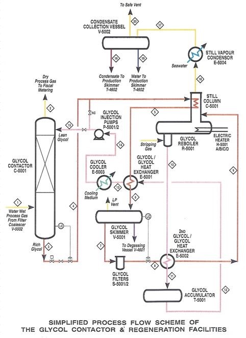
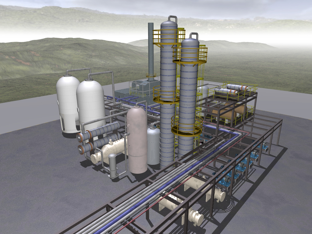
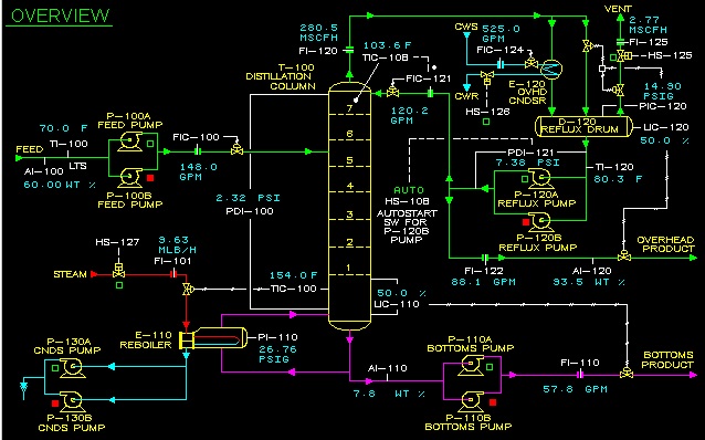
After retrieving natural gas from a well or reservoir, it still contains a substantial amount of water (liquid as well as vapor) and also some liquid carbohydrates (so-called condensates). This gas is often called wet gas and can cause several problems for downstream processes and equipment. So, before the natural gas is ready to be transported, water and condensates are removed from the gas in several steps. The Glycol Contactor is one of those steps. Glycol is a hygroscopic liquid which can easily absorb water vapor from a wet gas stream. So, by bringing the wet natural gas into contact with liquid glycol in a column, the last residues of water can be removed from the gas stream. Heating the glycol-water mixture in a Glycol Reboiler, will remove the absorbed water (by evaporation), such that the glycol can be regenerated and recycled. The picture below shows a simplified process flow scheme of the glycol contactor and regeneration facilities.

Hardware and Software Configuration

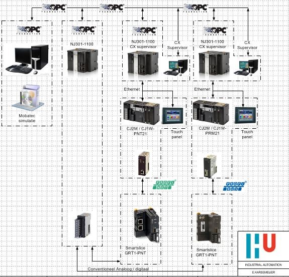
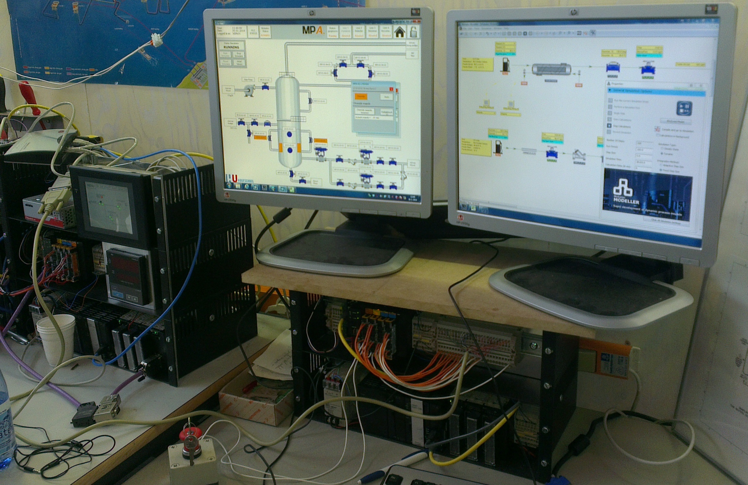
Since it was not possible for the students to realize a control setup on a real glycol dehydration unit (because such a unit was simply not available), one group of students was asked to make a real-time simulation of the process with Mobatec Modeller. Another group of students had the task to configure a real hardware PLC (Programmable Logic Controller) and configure an HMI (Human Machine Interface) and SCADA (Supervisory Control And Data Acquisition) with the available hardware and software. The simulation model should communicate via an OPC connection with a simulation-PLC.
The PLC’s were to be connected to the simulation-PLC in several ways:

• Via OPC (OLE for Process Control, OLE = Object Linking and Embedding)
• Direct via analog and digital IO-signals
• Via a Fieldbus and a remote IO-station with analog and digital IO-signals

The Assignment

The project was distributed amongst six groups, two of which was responsible for the simulation. The other four groups had to design a control (with slightly different specifications) for the system.

• The hardware and software configuration were thought out in big lines, but had to be designed and realized in detail by the different teams.
• The interface between the different systems, functional as well as technical, had to be determined by the teams themselves.
• The simulation of the process, including the assumptions and simplifications, had to be setup from scratch (using some building blocks). The simulation should have the option to create scenarios and “introduce errors”, such that the developed control strategies could be properly tested.
• Process conditions (under normal operation), process configuration details, battery limit (i.e. boundary) conditions and other relevant data were provided to the students, in order for them to make a realistic dynamic simulation model.
• The functional specification of the control system had to be designed by the teams.

The Modelling Effort

As a starting point for the modelling, the students had several P&ID’s (Piping and Instrumentation Diagrams) a PFD (Process Flow Diagram). The tags that were used in the P&ID’s were also used as names in the modelling environment, such that the coupling to the control PLC would be an easy task.
To build the model we provided the students with some basic (partially predefined) building blocks, since they had no background in Chemical Engineering. They had to refine and connect the building blocks and to tune the parameters to get trustworthy results. Especially the latter part, the tuning, can be quite time consuming for dynamic process models. Even more so if you do not have much experience in this field.
Obviously, since dynamic modelling was completely new for these students, some communication with Mobatec engineers was needed in order to get a good model. This interaction was kept to a minimum, however, and I was very pleased to learn how much these students were able to do themselves. Setting up and configuring the OPC connection, for example, didn’t require any interaction with us. They did this all by themselves, which is, of course, a positive outcome for both the students and Mobatec. Do you have any ideas or suggestions to make dynamic simulation a good learning tool for students? Or do you have other comments related to this topic?
Please feel free to post your experiences, insights and/or suggestions in the comment box below, such that we can all learn something from it.
To your success!
Mathieu.
———————————————–

The very first step in the process of obtaining a model is the mapping of the real-world prototype, the plant, into a mathematical object, alsocalled the primary model. This process is non-trivial because it involves structuring of the process into components and the application of a mapping theory for each component. Since the theories are context dependent, the structuring is tightly coupled to the theory chosen. The process of breaking the plant down to basic thermodynamic systems determines largely the level of details included in the model. It is consequently also one of the main factors for determining the accuracy of the description the model provides.
In previous blog posts I gave an idea on how a process can be broken down into smaller parts using only two basic building blocks, namely systems and connections. The resulting interconnected network of capacities is called the Physical Topology.
In another blog post the so-called Species Topology is discussed. This species topology is superimposed on the Physical Topology and defines which species and what reactions are present in each part of the physical topology.
Structuring is one factor determining the complexity of the model. Another factor comes to play when choosing descriptions for the various mechanisms such as extensive quantity transfer and conversion. For example in a distributed system, mass exchange with an adjacent phase may be modelled using a boundary layer theory or alternatively a surface renewal theory, to mention just two of many alternatives. The person modelling the process thus will have to make a choice. Since different theories result in different models, this implies making a choice between different models for the particular component. Structuring and use of theories will always imply intrinsic simplifying assumptions.
For example, modelling a heat transfer stream between the contents of the jacket and the contents of a stirred tank may be modelled using an overall heat transfer model, that is a pseudo-steady state assumption about the separating wall and the thermal transfer resistant of the fluids is made. Though, if one is interested in the dynamics of the wall, a simple lumping of the wall improves the description or, if this is still not sufficient, one may choose to describe the heat transfer using a series of distributed coupled system or a series of coupled lumped systems.
Assuming for the moment that the structuring is not causing any problems and assuming that a theory or theories are available for each of the components, the mapping into a mathematical object associated with a chosen view and an associated theory is formal.
The presumption is made that no other intrinsic assumptions are being made at this point, that is, the theory is applied in its purest form. Specifically, the conservation principles, which describe the basic behaviour of plants, are applied in their most basic form. Particularly the energy balance is formulated in terms of total energy and not in any derived state functions.
Once a mathematical model for the process components has been established, usually the next operation is to implement a set of assumptions which eliminate complete terms or parts thereof in the equations of the primary model. These are assumptions about the principle nature of the process such as no reaction, no net kinetic or potential energy gain or loss, no accumulation of kinetic or potential energy. Whilst not complete, this is a very typical set of assumptions applied on this level in the modelling process. The assumptions are of the form of definitions, that is variables, representing the terms to be simplified are instantiated. For example, the production term in the component mass balances might be set to zero.
Additional assumptions that simplify the process model may be introduced at any point in time. A very common simplification is the introduction of a pseudo-steady state assumption for a part of the process which essentially zeroes out accumulation terms and transmutes a differential equation into algebraic relation between variables. These can then be used to simplify the model by substitution and algebraic manipulation.
Our next blog post will discuss the implications that certain assumptions or constraints can have on an Equation Topology.
Are you aware of all the modelling assumptions you are making, when setting up a new model?
I invite to post your experiences, insights and/or suggestions in the comment box below, such that we can all learn something from it.
To your success!
Mathieu.
———————————————–

Process systems engineering spans the range between process design, operations and control. Whilst experiments are essential, modelling is one of the most important activities in process engineering, since it provides insight into the behaviour of the process(es) being studied.
In previous blogs we have been discussing particular uses of models and ways to setup consistent process models. But what kind of problems can, in general, be solved by mathematical models in Process Systems Engineering?

 

Three Principal Problems

The first step in identifying the various characteristic steps of Process Systems Engineering problem solving is to identify a minimal set of generic problems that are being solved. Most problems in this area have three major components, which are:
Model :: A realisation of the modelled system, simulating the behaviour of the modelled system.
Data :: Instantiated variables of the model. May be parameters that were defined or time records of input or output data obtained from an actual plant, marketing data etc.
Criterion :: An objective function that provides a measure and which, for example, is optimised giving meaning to the term best in a set of choices.
The particular nature of the problem then depends on which of these components is known and which is to be identified. Each type of problem is associated with a name which changes from discipline to discipline. The choice of the names listed below was motivated by the relative spread of the respective term in the communities. The following principle problems are defined: Simulation: Given model, given input data and given parameters find the output of the process.
Identification: Given model structure, sometimes several structures, given process input and output data, and a given criterion, find the best structure and the parameters for the parameterised model, where best is measured with the criterion.
Optimal Control: Given a plant model, a criterion associated with process input and process output, and the process characteristics, find the best input subject to the criterion.
The definition of simulation is straightforward. (It’s the core business of Mobatec 😉 ).
The task of identification though is not, in that it includes finding structure as well as parameters of a model. This in turn implies that many tasks match this description, such as process design and synthesis, controller design and synthesis, parameter identification, system identification, controller tuning and others fit this definition.
The definition of the optimal control task is also wider than one usually would project. Namely process scheduling and planning are part of this definition as well as the design of a shut-down sequence in a sequential control problem, to mention a few non-traditional members of this class.
In all three classes a model is involved. In this discussion parameterised input/output mapping are used because they are usually the type of model capturing the behaviour of a given system in the most condensed form. Though in each case it is solved for a different set of its components. In the case of the simulation, the outputs are being computed, in the case of the identification task, the best parameters are found and in the case of optimal control, the best input record is being determined.
In order to solve a problem, the model must be supplemented with a set of definitions, which, in combination with the model, define a mathematical problem that can be solved by a particular mathematical method. These definitions are instantiations of variables that assign known quantities to variables or functions of know quantities, where the functions may be arbitrarily nested. On this highest level, process engineering problem solving has four principle components:
1. Formulation of a model;
2. Problem specification;
3. Problem solution method;
4. Problem analysis.
Several blogs have already been devoted to model formulation, but it never hurts to rephrase and repeat a bit 😉
Models take a central position in all process engineering tasks as they replace the process for the analysis. They represent an abstraction of the process, though not a complete reproduction. Models make it possible to study the behaviour of a process within the domain of common characteristics of the model and the modelled process without affecting the original process. It is thus the common part, the homomorphism or the analogy between the process and model and sometimes also the homomorphism between the different relations (= theories) mapping the process into different models that are of interest. The mapping of the process into a model does not only depend on the chosen theory, but also on the conditions under which the process is being viewed. The mapped characteristics vary thus not only with the applied theory but also with the conditions.
Different tasks focus on different characteristics and require different levels of information about these characteristics. For example control would usually be achievable with very simple dynamic models, whilst the design of a reactor often requires very detailed information about this particular part of the process. The result is not a single, all-encompassing model but a whole family of models. In fact, there is no such thing as a unique and complete model, certainly not from the philosophical point of view nor from a practical, as it simply reflects the unavoidable inability to accumulate complete knowledge about the complex behaviour of a real-world system. More practically and pragmatically a process is viewed as the representation of the essential aspects of a system, namely as an object, which represents the process in a form useable for the defined task. Caution is advised, though, as the term essential is subjective and may vary a great deal with people and application.
The term multi-faceted modelling has been coined reflecting the fact that one deals in general with a whole family of models rather than with a single model. Whilst certainly the above motivation is mainly responsible for the multi-faceted approach, solution methods also have use for a family of models as they can benefit from increasing the level of details in the model as the solution converges. An integrated environment must support multi-faceted modelling, that is mapping of the process into various process models, each reflecting different characteristics or the same characteristics though with different degree of sophistication and consequent information contents.
In the next blog post we will zoom into the assumptions that are made when making a model and the implication these assumptions can have on the end result.
To your success!
Mathieu.
———————————————–

According to the definition on Wikipedia “Serious Games are simulations of real-world events or processes designed for the purpose of solving a problem. Although serious games can be entertaining, their main purpose is to train or educate users, though it may have other purposes, such as marketing or advertisement. Serious game will sometimes deliberately sacrifice fun and entertainment in order to achieve a desired progress by the player. Serious games are not a game genre but a category of games with different purposes. This category includes some educational games and advergames, political games, or evangelical games. Serious games are primarily focused on an audience outside of primary or secondary education.”
In this month’s blog I would like to start a discussion about the usefulness of Serious Games within Chemical Engineering education and in the Process Industry.
In my opinion, one of the best ways for a new operator to learn the ins and outs of a plant he started working with, is to let him solve all kinds of real problems or situations that can occur during operation of the plant. Since a real plant normally runs very stable for long periods of time, it’s not very convenient to let an operator “play” with the real plant. A very good alternative would be to have a high-fidelity Operator Training Simulator to learn the process.
Operator Training Simulators can be seen as a first generation of Serious Games for chemical engineers and have already been around for decades. They started out as hardware-based solutions, but in the 1980s OTS applications became available for PCs. In the last decade a new innovation became available: A virtual reality component showing the outside operator view. This 3D world is dynamically linked to the process simulator. With a 3D visualization a “Virtual Outside Operator” can actually open and close hand-operated valves, start and stop pumps, take field reading, see and hear equipment running, communicate with the control room, etc.. Instructors can mentor and manage training sessions, instead of being tied up in role playing the functions of an Outside Operator of previously provided “remote function” switches.
At Mobatec we also have several years of experience of linking (real-time) dynamic process models to 3D visual plants. The 3D graphics are developed for us by the high-tech company ExplainMedia. Have a look at the short video if you are not sure what a 3D visualization of a plant is. I regularly show interactive examples of these very attractive and intuitive, dynamic 3D modules to lecturers at Chemical Engineering departments or technical staff of a chemical plant and initially they react very enthusiastically. However, when talking a bit longer to get a feel for if they would be interested in having such a 3D module from their own environment, they usually become more reluctant.
A feedback I often get when talking to these people is that adding a 3D world to the education or training modules would be a “nice to have”, but not a “must”. Which, of course, typically translates to “we would really like to have it, but it must be cheap!”. However, realizing a cheaper solution for industry, especially when looking at education, would also imply/ have as a side-effect that a lot Universities and Schools should be potentially interested in 3D modules. Otherwise it would not be worth the investment.
I am very interested in your view on this subject:
“Are interactive 3D visualizations of (parts of) chemical processes a valuable addition to a Chemical Engineering education and/ or learning tools of processing plants?”
I invite to post your comments, insights and/or suggestions in the comment box below.
To your success!
Mathieu.
———————————————–

In this month’s blog I will attempt to present a “roadmap” for constructing structurally consistent and solvable dynamic process models. I tried to keep it short and simple, but I soon realised that this was nearly impossible, since leaving out certain details would make it difficult for a reader to grasp the complete picture.
So, this blog is a bit longer than usual. But if you take the time to consume it, you will certainly get more insight in how to properly set up a correct, structurally solvable dynamic process model (using any equation based solver).
A more thorough discussion on this subject is given in the document “Concepts and Modelling Methodology”. Just click on the link to download a copy.
 

In order to characterize the behaviour of a process, information is needed about the natural state of this process (at a given time) and about the change of this state with time. The natural state of a process can be described by the values of a set of fundamental extensive quantities, while the change of state is given by the balance equations of those fundamental variables.
The fundamental extensive variables represent the ”extent” of the process c.q. the quantities being conserved in the process. In other words: they represent quantities for which the conservation principle and consequently also the superposition principle applies. So, for these variables, the balance equations are valid. In most chemical processes, the fundamental variables are: component mass, total energy and (sometimes) momentum.
The dynamic behaviour of a system can be modelled by applying the conservation principles to the fundamental extensive quantities of the system. The principle of conservation of any extensive quantity (x) of a system states that what gets transferred into the system must either leave again or is transformed into another extensive quantity or must accumulate in the system (In other words: no extensive quantity is lost).
In my PhD thesis I showed that the dynamic part (i.e. the differential equations) of physical-chemical-biological processes can be represented in a concise, abstract canonical form, which can be isolated from the static part (i.e. the algebraic equations). This canonical form, which is the smallest representation possible, incorporates very visibly the structure of the process model as it was defined by the person who modelled the process: The system decomposition (physical topology) and the species distribution (species topology) are very visible in the model definition. The transport (z) and production (r) rates always appear linearly in the balance equations, when presented in this form:

dx/dt = Az+ Br

in which:

• x :: Fundamental state vector (Primary State vector)
• z :: Flow of extensive quantities (Transport rates)
• r :: Kinetics of extensive quantity conversion (Reaction rates)
• A :: Interconnection matrix
• B :: Stoichiometric coefficient matrix

  The classification of variables that is presented here is, in the first place, based on the structural elements of the modelling approach (namely systems and connections).
The matrices A and B are completely defined by the model designer’s definition of the physical and species topology of the process under investigation. Therefore these matrices are trivial to setup (and are actually automatically constructed by Mobatec Modeller). The only things a model designer has to do to complete the model are:

• Provide a link between the transport and reaction rate vectors and the primary state vector. Each element in the transport and reaction rate vectors has to be (directly or indirectly) linked to the primary state vector. This “linking” is done with one or more algebraic equations. If certain elements of the rate vectors are not defined in the algebraic equations, the mathematical system will have too many unknowns and can consequently not be solved.
• Give a mapping which maps the primary state of each system in a secondary state. This mapping is necessary because usually transport and reaction rates are defined as functions of secondary state variables (a heat flow can, for example, be expressed as a function of temperature difference).

 

Algebraic Equations

So, in addition to the balance equations, we need other relationships to express thermodynamic equilibria, reaction rates, transport rates for heat, mass, momentum, and so on. Such additional relationships are needed to complete the mathematical modelling of the process. A model designer should be allowed to choose a particular relationship from a set of alternatives and to connect the selected relationship to a balance equation or to another defined relationship. The algebraic equations are divided into three main classes, namely system equations, connection equations and reaction equations.
 

System Equations

For each system that is defined within the physical topology of a process, a mapping is needed which maps the primary state variables (x) into a set of “secondary state” variables (y = f(x)). The primary states of a system are fundamental quantities for describing the behaviour of the system. The fundamental state is defined intrinsically through the fundamental behaviour equations. The application of fundamental equations of component mass and energy balances intrinsically defines component mass and energy as the fundamental state variables. Alternative state variables are required for the determination of the transfer rate of extensive quantities and their production/consumption rate.
The equations that define secondary state variables do not have to be written in explicit form, by the way, but it has to be possible to solve the equations (either algebraically or numerically) such that the primary state can be mapped into the secondary state. This means that each defined equation has to define a new variable. Equations that link previously defined variables together are not allowed, since the number of equation would then exceed the number of variables and the set of equations of this system would thus be over-determined.
 

Connection Equations

The flow rates (z), which emerge in the balance equations of a system, represent the transfer of extensive quantities to and from adjacent systems. These flow rates can be specified or linked to transfer laws, which are usually empirical or semi-empirical relationships. These relationships are usually functions of the states, and the physical and geometrical properties of the two connected systems. For example, the rate of conductive heat transfer Q through a surface A between two objects with different temperatures can be given by:

Q = U * A *(T_or-T_tar)

This relationship depends on the temperatures T_or and T_tar of the origin and target object respectively. Temperature is of course a (secondary) state variable. The rate of heat transfer also depends on the overall heat transfer coefficient U, which is a physical property of the common boundary segment between the two systems, and on the total area of heat transfer A, which is a geometrical property.
A transfer law thus describes the transfer of an extensive quantity between two adjacent systems (z = f(yor, ytar)). The transfer rate usually depends on the state of the two connected systems and the properties of the boundary in between.
 

Reaction Equations

Depending on the time scale of interest, we can divide reactions into three groups:

• Very slow reactions (slow in the measure of the considered range of time scales). These reactions do not appreciably occur and may be simply ignored.
• Reactions that occur in the time-scale of interest. For these reactions kinetic rate laws can be used.
• Very fast reactions (relative to the considered time scale), for which is assumed that the equilibrium is reached instantaneously.

  As the non-reactive parts do not further contribute to the discussion, they are left out in the sequel. The fast (equilibrium) reactions go beyond the scope of this blog and are therefore also not discussed.
For the “normal” reactions the reaction rates of the reactions in the relevant times scale must be defined by kinetic rate equations. The production terms are linked to kinetic laws, which are empirical equations. They are usually written as a function of a set of intensive quantities, such as concentrations, temperature and pressure (r = f(y_sys)). For example, the reaction rate r of a first-order reaction taking place in a lump is given by:

r = V * k₀ * exp(-E/(R * T))*c_a

where:

• r :: Reaction rate of a first-order reaction
• V :: Volume of the system
• k₀ :: Pre-exponential kinetic constant
• E :: Activation energy for the reaction
• R :: Ideal gas constant
• T :: Temperature of the reacting system
• C_a :: Concentration of component A in the system

  Temperature and concentration(s) of the reactive component(s) are state variables (y) of the reactive system. Reaction constants and their associated parameter such as activation energy and pre-exponential factors are physical properties. In some cases, also geometrical properties of the system are part of the definition of the kinetic law, such as the porosity or other surface characterizing quantities.

Consclusions

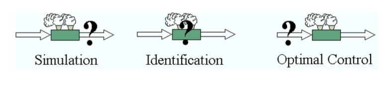
When a dynamic process model is formulated and proper initial conditions have been defined, then the information flow of a simulation can be depicted as in the above figure. Starting from the initial conditions x₀, the secondary state variables y of all the systems can be calculated (via the System Equations y=f(x)). Subsequently, the flow rates z of all the defined connections and the reaction rates r of all the defined reactions can be calculated (z = f(y_or, y_tar); r = f(y_sys)). These rates are the inputs of the balance equations, so now the integrator can compute values for the primary state variables x on the next time step. With these variables, the secondary state y can be calculated again and the loop continues until the defined end time is reached.
To put it in other words: A model designer should only be concerned with the algebraic equations (the right hand side of the figure), which means that the primary state variables x of each system can be considered as “known”. Systems are only interacting with each other through connections and therefore the calculation of the secondary variables of each system can be done completely independent of other systems.
The system equations map the primary state x into a secondary state y for each individual system, and each defined equation has to define a (secondary) variable. In some cases two or more equations may introduce two or more new variables, such that these equations have to be solved simultaneously in order to get a value for the variables.
For connection and reaction equations a similar conclusion can be drawn. For these equations the secondary variables of the systems (y) can be considered as “known”.
Looking at modelling like this, makes it a lot easier than trying to understand/debug the complete model of a process. Just divide your model into systems and connections, assign equations to those objects (typically not more than 10) and solve any problem that arises per object. Resolving a problem (or even several) of about 10 equations is a lot easier than when hundreds or more are considered at the same time!
Do you have experience with making (large) dynamic process models?
I invite to post your experiences, insights and/or suggestions in the comment box below, such that we can all learn something from it.
To your success! Mathieu.
———————————————–