In the blog post of last month we discussed about the substitution of variables and whether these variable transformation are actually necessary to solve the problems at hand. Part of the discussion was concerned with the computational causality of the involved equations and this month I would like to spend a few more words on that topic.
As discussed in previous blog posts, the dynamic part (i.e. the differential equations) of a process model can be isolated from the static part (i.e. the algebraic equations). The dynamic part can be trivially derived from the model designer’s definition of the Physical Topology and Species Topology of the process. The static part has to be defined by the physical insight of the model designer.
For each modelling object (i.e. system, connection or reaction) the algebraic equations can, in principle, be chosen “randomly” from a database. In doing so, the problem arises that not every numerical equation solver will be able to solve the equations, since the equations are not in the so-called correct computational order and are not always in (correct) explicit form. Nowadays, many solvers (so-called DAE-1 solvers) can easily handle implicit algebraic equations, but when the equations are re-ordered and simplified by performing preliminary symbolic manipulations, a more efficient computational code could be obtained.
If you are using an explicit solver (such as Matlab) to solve your model equations, an important step to achieve an efficient computational code for DAEs, is to solve the equations for as many algebraic variables as possible. This way it is not necessary to introduce these variables as unknowns in the numerical DAE-solver, since they can be calculated at any call of the residual routine from the information available.
Consider the simple pair of equations:

y – 2x = 4  (1)

x – 7 = 0    (2)

In order to solve these equations directly, they must be rearranged into the form:

x = 7          (3)

y = 2x + 4  (4)

The implicit equation (2) cannot readily be solved for x by a numerical program, whilst the explicit form, namely (3), is easily solved for and only requires the evaluation of the right-hand-side expression. Equation (1) is rearranged to give (4) for y, so that when x is known, y can be calculated.
The rearranged form of the set of equations can be solved directly because it has the correct computational causality. As discussed in the blog on substitution, this computational causality is, quite obviously, not a physical phenomenon, but a numerical artefact. Take, for example, the ideal gas law:

pV = nRT

This is a static relation, which holds for any ideal gas. This equation does not describe a cause-and-effect relation. The law is completely impartial with respect to the question whether at constant temperature and constant molar mass a rise in pressure causes the volume of the gas to decrease or whether a decrease in volume causes the pressure to rise. For a solving program, however, it does matter whether the volume or the pressure is calculated from this equation.
It is rather inconvenient that a model designer must determine the correct computational causality of all the algebraic equations that belong to each modelling object, given a particular use of the model (simulation, design, etc.). It is much easier if the equations could just be described in terms of their physical relevance and that a computer program automatically determines the desired causality of each equation and solves each of the equations for the desired variable, for example by means of symbolic manipulation or implicit solving.
Whether the entered equations are in the correct causal form or not, they always have to adhere to some conditions:

• For any set or equations to be solvable, there must be exactly as many unknowns as equations.
• It must be possible to rearrange the equations such that the system of equations can be solved for all unknowns.

The first condition, called the Regularity Assumption, is obviously a necessary condition. It can be checked immediately and all numerical DAE solvers take this preliminary check.
In order to solve a set of equations efficiently, the equations must be rearranged in Block Lower Triangular (BLT) form with minimal blocks, which can be solved in a nearly explicit forward sequence. 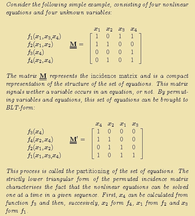Several efficient algorithms exist to transform to block lower triangular form. Many references state that it is, in general, not possible to transform the incidence matrix to a strictly lower triangular form, but that there are most likely to be square blocks of dimension > 1 on the diagonal of the incidence matrix. These blocks correspond to equations that have to be solved simultaneously. 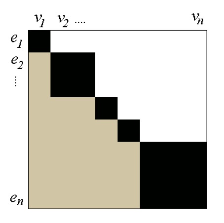In the above figure the incidence matrix of a set of equations (e), which are transformed to BLT form, is shown. White areas indicate that the variables (v) do not appear in the corresponding equation, grey areas that they may or may not appear, and black areas represent the variables still unknown in the block and which can be computed from the corresponding equations. So, a block of this matrix indicates which set of variables can be computed if the previous ones are known.
Although it is good to know about computational causality, a model designer does, in general, not have to worry about BLT forms, because most equation based solvers (Mobatec Modeller included) handle this automatically.
The BLT format is used by these solvers to define which variable should be solved from which equation. Only in the case two (or more) variables have to be solved from two (or more) equation, a user input could, in some cases, be required, since a “computer guess” could lead to a (numerically) non-optimal choice.
“Did you ever have to deal with the computational order of your equations? Does your solver do the sorting automatically, but sometimes makes a “bad” choice (maybe without you being aware of it)?”
I invite to post your comments, insights and/or suggestions in the comment box below.
To your success!
Mathieu.
———————————————–