

|

Posted on:
31 Jan 2014
|
Physical topologies are the abstract representation of the containment of the process in the physical sense. They visualise the principle dynamic contents of the process model and therefore the construction of a physical topology is the most fundamental part of the modelling process. Any changes in the physical topology will substantially affect the structure and contents of the final model.
The structuring of the process implements the first set of assumptions in the modelling process. The resulting decomposition is, in general, not unique. However, the resulting model depends strongly on the choice of the decomposition. As a rule: the finer the decomposition, the more complex will the resulting model be.
The decision of defining subsystems is largely based on the phase argument, where the phase boundary separates two systems. The second decision criterion utilises the relative size of the capacities and the third argument is based on the relative velocity with which subsystems exchange extensive quantities. Another argument is the location of activities such as reactions. The relative size of the model components, measured in ratios of transfer resistance and capacities, termed time constants, is referred to as “granularity”. A large granularity describes a system cruder, which implies more simply, than a model with a finer granular structure. It seems apparent that one usually aims at a relative uniform granularity, as these systems are best balanced and thus more conveniently solved by numerical methods.
Models of different granularity help in analysing the behaviour of the process in different time scales. The finer the granularity, the more the dynamic details and thus the more of the faster effects are captured in the process description. Since each model is constructed for a specific goal, a process model should reflect the physical reality as accurately as needed. The accuracy of a model intended for numerical simulation, for example, should (in most cases) be higher than the accuracy of a model intended for control design.
To illustrate the concepts mentioned above, consider the following example concerning a stirred tank reactor:
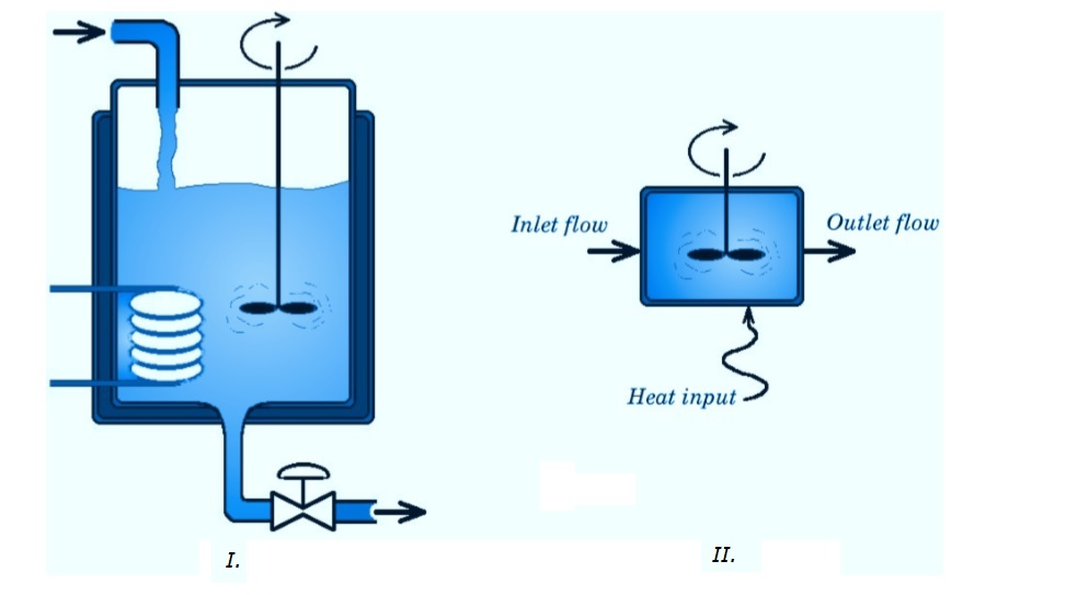 Figure I shows a stirred tank reactor, which consists of an inlet and outlet flow, a mixing element, a heating element and liquid contents. If the model of this tank is to be used for a rough approximation of the concentration of a specific component in the outlet flow or for the liquid-level control of the tank, a simple model suffices. The easiest way to model this tank is to view it as an ideally stirred tank reactor (ISTR) as shown in figure II. This implies that a number of assumptions have been made regarding the behaviour and properties of the tank. The most important assumption is the assumption that the contents of the tank is ideally mixed and hence displays uniform conditions over its volume. Another assumption can be that heat losses to the environment are negligible.
After making these and maybe some more assumptions, the modeller can write the component mass balances and the energy balance of the reactor. With these equations and some additional information (e.g. kinetics of reaction, physical properties of the contents, geometrical relations, state variable trans- formations, etc.) the modeller can describe the dynamic and/or static behaviour of the reactor.
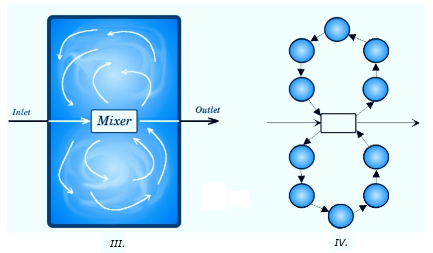 If the tank has to be described on a much smaller time-scale and/or the behaviour of the tank has to be described in more detail, then the ISTR model will not suffice. A more accurate description often asks for a more detailed model. In order to get a more detailed description the modeller could, for example, choose to try to describe the mixing process in the tank (see figure III). Figure IV shows a possible division of the contents of the tank into smaller parts. In this drawing a circle represents a volume element which consists of a phase with uniform conditions. Each volume element can thus be viewed as an ISTR. The arrows represent the mass flows from one volume to another. In order to describe the behaviour of the whole tank, the balances of the fundamental extensive quantities (component mass and energy usually suffice) must be established for each volume element. The set of these equations, supplemented with information on the extensive quantity transfer between the volumes and other additional information, will constitute the mathematical description of the dynamic and/or static behaviour of the reactor.
The model of the mixing process could, of course, be further extended to get a more accurate description. The number of volume elements could for example be increased or one could consider back mixing or cross mixing of the liquid between the various volume elements (In principle, if one increases the complexity of this description, one approaches the type of models that result from approximating distributed models using computational fluid dynamic packages). The conduction of heat to each volume could also be modelled. One could model a heat flow from a heating element to each volume, or only to those volume elements which are presumed to be the nearest to the heating element, etc. As one may imagine there are many ways to describe the same process. Each way usually results in a unique mathematical representation of the behaviour of the process, depending on the designers view on and knowledge of the process, on the amount of detail he wishes to employ in the description of the process and, of course, on the application of the model.
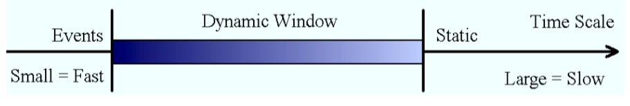
When employing the term time scale, we use it in the context of splitting the relative dynamics of a process or a signal (the result of a process) into three parts, namely a central interval where the process or signal shows a dynamic behaviour (1). This dynamic window is on one side guarded by the part of the process that is too slow to be considered in the dynamic description, thus is assumed constant (2). On the other side the dynamic window is attaching to the sub-processes that occur so fast that they are abstracted as event – they just occur in an instant (3). Any process we consider requires these assumptions and it is the choice of the dynamic window that determines largely the fidelity of the model in terms of imaging the process dynamics.
 One may argue that one should then simply make the dynamic window as large as probably possible to avoid any problems, which implies an increase in complexity. Philosophically all parts of the universe are coupled, but the ultimate model is not achievable. When modelling, a person must thus make choices and place focal points, both in space as well as in time. The purpose for which the model is being generated is thus always controlling the generation of the model. And the modeller, being the person establishing the model, is well advised to formulate the purpose for which the model is generated as explicit as possible.
A window in the time scales must thus be picked with the limits being zero and infinity. On the small time scale one will ultimately enter the zone where the granularity of matter and energy comes to bear, which limits the applicability of macroscopic system theory and at the large end, things get quite quickly infeasible as well, if one extends the scales by order of magnitudes. Whilst this may be discouraging, having to make a choice is usually not really imposing any serious constraints, at least not on the large scale. Modelling the movement of tectonic plates or the material exchange in rocks asks certainly for a different time scale than modelling an explosion, for example. There are cases, where one touches the limits of the lower scale, that is, when the particulate nature of matter becomes apparent. In most cases, however, a model is used for a range of applications that usually also dene the relevant time-scale window.
The dynamics of the process is excited either by external effects, which in general are constraint to a particular time-scale window or by internal dynamics resulting from an initial imbalance or internal transposition of extensive quantity. Again, these dynamics are usually also constraint to a time-scale window. The maximum dynamic window is thus the extremes of the two kinds of windows, that is, the external dynamics and the internal dynamics.
A “good” or “balanced” model is in balance with its own time scales and the time-scale within which its environment operates. In a balanced model, the scales are adjusted to match the dynamics of the individual parts of the process model. Balancing starts with analysing the dynamics of the excitations acting on the process and the decision on what aspects of the process dynamics are of relevance for the conceived application of the model. What has been defined as a system (capacity) before may be converted into a connection later and vice versa as part of the balancing process. This makes it difficult, not to say impossible, to define systems and connections totally hard. The situation clearly calls for a compromise, which, in turn, opens the door for suggesting alternative compromises. There is not a single correct choice and there is certainly room for arguments but also for confusion. Nevertheless a decision must be taken.
Initially one is tempted to classify systems based on their unique property of representing capacitive behaviour of volumes, usually also implying mass. In a second step one may allow for an abstraction of volumes to surfaces, because in some applications it is convenient to also abstract the length scale describing accumulation to occur inside, so-to-speak, or on each side of the surface.
What is your experience with time scale assumptions? Where you aware that you actually always make them, when modelling? Are you aware of the effect they have on your end results?
I invite to post your experiences, insights and/or suggestions in the comment box below, such that we can all learn something from it.
To your success!
Mathieu.
———————————————–
The structuring of the process implements the first set of assumptions in the modelling process. The resulting decomposition is, in general, not unique. However, the resulting model depends strongly on the choice of the decomposition. As a rule: the finer the decomposition, the more complex will the resulting model be.
The decision of defining subsystems is largely based on the phase argument, where the phase boundary separates two systems. The second decision criterion utilises the relative size of the capacities and the third argument is based on the relative velocity with which subsystems exchange extensive quantities. Another argument is the location of activities such as reactions. The relative size of the model components, measured in ratios of transfer resistance and capacities, termed time constants, is referred to as “granularity”. A large granularity describes a system cruder, which implies more simply, than a model with a finer granular structure. It seems apparent that one usually aims at a relative uniform granularity, as these systems are best balanced and thus more conveniently solved by numerical methods.
Models of different granularity help in analysing the behaviour of the process in different time scales. The finer the granularity, the more the dynamic details and thus the more of the faster effects are captured in the process description. Since each model is constructed for a specific goal, a process model should reflect the physical reality as accurately as needed. The accuracy of a model intended for numerical simulation, for example, should (in most cases) be higher than the accuracy of a model intended for control design.
To illustrate the concepts mentioned above, consider the following example concerning a stirred tank reactor:
After making these and maybe some more assumptions, the modeller can write the component mass balances and the energy balance of the reactor. With these equations and some additional information (e.g. kinetics of reaction, physical properties of the contents, geometrical relations, state variable trans- formations, etc.) the modeller can describe the dynamic and/or static behaviour of the reactor.
The model of the mixing process could, of course, be further extended to get a more accurate description. The number of volume elements could for example be increased or one could consider back mixing or cross mixing of the liquid between the various volume elements (In principle, if one increases the complexity of this description, one approaches the type of models that result from approximating distributed models using computational fluid dynamic packages). The conduction of heat to each volume could also be modelled. One could model a heat flow from a heating element to each volume, or only to those volume elements which are presumed to be the nearest to the heating element, etc. As one may imagine there are many ways to describe the same process. Each way usually results in a unique mathematical representation of the behaviour of the process, depending on the designers view on and knowledge of the process, on the amount of detail he wishes to employ in the description of the process and, of course, on the application of the model.
When employing the term time scale, we use it in the context of splitting the relative dynamics of a process or a signal (the result of a process) into three parts, namely a central interval where the process or signal shows a dynamic behaviour (1). This dynamic window is on one side guarded by the part of the process that is too slow to be considered in the dynamic description, thus is assumed constant (2). On the other side the dynamic window is attaching to the sub-processes that occur so fast that they are abstracted as event – they just occur in an instant (3). Any process we consider requires these assumptions and it is the choice of the dynamic window that determines largely the fidelity of the model in terms of imaging the process dynamics.
A window in the time scales must thus be picked with the limits being zero and infinity. On the small time scale one will ultimately enter the zone where the granularity of matter and energy comes to bear, which limits the applicability of macroscopic system theory and at the large end, things get quite quickly infeasible as well, if one extends the scales by order of magnitudes. Whilst this may be discouraging, having to make a choice is usually not really imposing any serious constraints, at least not on the large scale. Modelling the movement of tectonic plates or the material exchange in rocks asks certainly for a different time scale than modelling an explosion, for example. There are cases, where one touches the limits of the lower scale, that is, when the particulate nature of matter becomes apparent. In most cases, however, a model is used for a range of applications that usually also dene the relevant time-scale window.
The dynamics of the process is excited either by external effects, which in general are constraint to a particular time-scale window or by internal dynamics resulting from an initial imbalance or internal transposition of extensive quantity. Again, these dynamics are usually also constraint to a time-scale window. The maximum dynamic window is thus the extremes of the two kinds of windows, that is, the external dynamics and the internal dynamics.
A “good” or “balanced” model is in balance with its own time scales and the time-scale within which its environment operates. In a balanced model, the scales are adjusted to match the dynamics of the individual parts of the process model. Balancing starts with analysing the dynamics of the excitations acting on the process and the decision on what aspects of the process dynamics are of relevance for the conceived application of the model. What has been defined as a system (capacity) before may be converted into a connection later and vice versa as part of the balancing process. This makes it difficult, not to say impossible, to define systems and connections totally hard. The situation clearly calls for a compromise, which, in turn, opens the door for suggesting alternative compromises. There is not a single correct choice and there is certainly room for arguments but also for confusion. Nevertheless a decision must be taken.
Initially one is tempted to classify systems based on their unique property of representing capacitive behaviour of volumes, usually also implying mass. In a second step one may allow for an abstraction of volumes to surfaces, because in some applications it is convenient to also abstract the length scale describing accumulation to occur inside, so-to-speak, or on each side of the surface.
What is your experience with time scale assumptions? Where you aware that you actually always make them, when modelling? Are you aware of the effect they have on your end results?
I invite to post your experiences, insights and/or suggestions in the comment box below, such that we can all learn something from it.
To your success!
Mathieu.
———————————————–