Events and Discontinuities

 Thumbnail
Mathieu Westerweele
Mathieu Westerweele
Posted on:
31 Jul 2014
The dynamic behaviour of a process can be abstracted to the point at which it can be represented by the smooth, continuous change of a series of state variables. This allows such a process to be represented mathematically as a set of DAEs.
The majority of processes, however, cannot be considered entirely continuous, but also experience significant discrete changes or discontinuities superimposed on their predominantly continuous behaviour. Such discrete changes, often referred to as events, can either be planned changes, called time events (for example, planned operational changes, such as start-up and shut-down, feed stock and/or product changes, process maintenance, switching a valve) or non-planned changes, called state events (overflow of a tank, (dis)appearance of a phase, inversion of a flow).
The exact time of occurrence of time events is either known a priori or it can be computed from the occurrence of a previous event. The time of occurrence of state events is not known in advance because it depends on the system fulfilling certain state conditions.
In addition to the two types of events we can classify events in another way, namely in events that do not change the (dynamic) model structure and events that change the (dynamic) model structure. With events that do not change the model structure, the balance equations are not altered, but some algebraic equations are changed. This usually results in a non-smooth continuation of the primary state variables.
———————————————————————————-
Example: Tank with Fast and Equilibrium Reaction Consider a tank with an inlet (consisting of two components A and B) and an outlet. The contents of the tank consist of four components (A, B, C and D) among which two fast reactions occur, namely:
A + B → C  (1)
A ↔ D        (2)
The first reaction (1) is a very fast, one way reaction. This means that there is no measurable inverse reaction and one of the two components A or B will always be completely consumed (i.e.: n_A =0 or n_B =0). The other reaction (2) is an equilibrium reaction, which means that there will always be a certain ratio between components A and D (c_A = k ∗ c_D). Because both reactions are fast in the context of the viewed time scale, the reaction terms that appear in the balance equations can be removed be using the Simple Index Reduction Algorithm (as discussed in previous blogs).
Reaction
Figure: Simulation of a tank in which a fast and an equilibrium reaction take place.
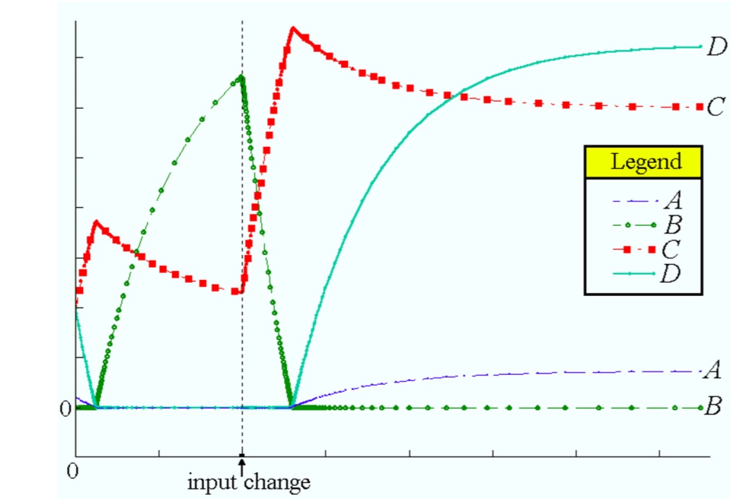
The figure shows the result of a simulation of the tank. In this figure we can see three events taking place.
At the start of the simulation there is an excess of A in the tank, which means that there will be no B, since all B that is available directly reacts with A to form C. The inlet flow contains more B than A and this results in diminishing quantities of A (and, consequently, D) in the tank until the amount of A (and D) in the tank reaches zero. At this point we encounter the first event, for now there will be an excess of B available in the tank and A (and D) will be non-existent.
At a certain point in time the input is changed such that the inlet flow will contain more A than B. A second event is the result. The amount of B will decrease until it reaches zero. This will initiate the third event, such that A (and D) will be present again.
Obviously, the first and last event were state events, while the second event was a time event.

———————————————————————————-
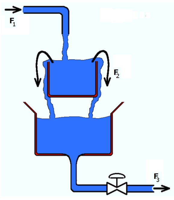
In our Modelling Methodology the model structure is typically never changed when an event occurs. Special IF-THEN-ELSE equations are used to describe state-dependent events. As an example, consider the overflow equation that was mentioned in our blog post on the Overflowing Tank:
F2:  IF V > Vmax THEN
         F2 = K * (V – Vmax)
       ELSE
         F2 = 0
       END
Instead of changing the balance equations when there is no overflow (if the volume in the tank is lower than the maximum volume Vmax), the value of the overflow is simply set to zero.
For those who are interested in the simultaneous solving of (large) mathematical sets of differential and algebraic equations (DAE) that also include conditional statements (IF-THEN-ELSE type equations), it should be noted that the conditions are checked before a calculation step is performed. So, with the information of the previous time step it is determined which equations are used for solving the DAE. The effect of a state-dependent conditional statement is, therefore, typically “too late” if the calculation step is too large. This effect can give rise to “interesting” modelling results and should be well understood when making dynamic models. I will most likely discuss it in another blog post ;).
What is your experience with events and discontinuities in your models? Did you ever run into unexpected model behaviour because of these events?
I invite to post your experiences, insights and/or suggestions in the comment box below, such that we can all learn something from it.
To your success!
Mathieu.
———————————————–

Steady-State Assumptions

 Thumbnail
Mathieu Westerweele
Mathieu Westerweele
Posted on:
30 June 2014
Last month we had a look at modelling challenges that can arise when making constraining assumptions. This month’s blog will cover a related form of constraining assumptions, the steady-state assumption.
The need for (pseudo) steady-state assumptions may arise for different reasons. Often the purpose is to either simplify the dynamic behaviour of the system by idealising components or it is to compensate for information that is not readily available or difficult to model for other reasons.
The idealisation of components is context-wise related to the subject of singular perturbation. Since the model is built for a specific purpose, one may choose to ignore the dynamic effects of certain parts of the system and assume that they are either extremely slow thus can be approximated as reservoir providing an infinite-size source of matter, energy, etc., or one may make assumptions of instantaneous dynamics for small-capacity parts.
If you critically analyse models, as they are published in the literature, you will find that such assumptions are omnipresent. In fact they are intrinsically in the basics as models are mostly build on the assumption of reversibility, which does imply that one deals with small capacity elements that move along trajectories on the equilibrium surface.
One often finds problems where two systems of largely different nature are coupled. For example a large system that is connected to a small system. Often the dynamic effects of the small system may be ignored, but very often too, the small system makes all the difference. Models in which a phase transition takes place are of this nature in that the phase boundary separating the two phases is very important when describing the flow of mass from one phase to another. This concept may also be applied to time scales, such as fast and slow systems. For these systems the singular perturbation theory is applicable. For fast systems a pseudo steady-state assumption is made:

ε dx/dt = A z + B r


which yields

0 = A z + B r

if ε := 0.
The capacity effects of the fast systems are omitted and this reduces the state of the process because the dynamic equations of this parts are set to zero. The state of a fast capacity becomes a function of the state of its environment, which mathematically reflects into the elimination of the state. So, for these fast systems the accumulation terms vanish and, consequently, the primary state variables are undefined for these systems. The balance equations of the fast systems are still valid and are used to calculate undefined variables either directly or indirectly. Quite obviously, an “unmodelled flow” can be calculated directly via a steady-state assumption.
In general, a number of steady-state assumptions that remove n states result in the following set of algebraic equations (only for the fast capacities; see the blog post on structurally consistent models for a notion of what these equations and variables represent):

0 = A z + B r


y = f(x)


z = g(y, ye)


r = h(y)

from which n variables (either flow rates (z), reaction rates (r) and/or states (x or y)) can be calculated (less variables can be calculated when index reduction algorithms affect the steady-state balance equations). In this set the ye represent the (secondary) states of the environment systems (i.e. systems that are connected to the steady-state systems) and are the driving forces of the algebraic equations. A bipartite graph analysis could provide the means for finding the different sets of variables that can be computed from this set of algebraic equations. Normally, though, each steady-state assumption can be handled locally and it is clear for which variables the equations are solved.
Consider the following example of a simple heat flow though a thin wall:
Heat Flow
Figure A: simple process; a heat flow through a thin wall.
Figure B: (possible) Physical topology of this simple process
Three systems are interconnected via heat connections. The enthalpy balance of the middle system (2) of figure B is:

d(H)/dt = qa − qb

If the second flow (qb) remains “unmodelled”, then a steady-state assumption (on system 2: d(H)/dt := 0) can be made to calculate this flow via the balance equation:

qa = qb

If there would have been no inlet flow to system 2 and a steady- state assumption is made, this would, of course, result in no flow through connection 2 (i.e. qb = 0).
As mentioned, the steady-state assumption essentially makes the state of a system a function of the state of its environment. The state of the environment can thus be used to redefine the (secondary) state (i.e. the intensive quantities) of the system.
Consider figure B once again. The heat ows through the connections a and b are now defined as functions of the temperatures of the interconnected systems:

qa = U1 A1 (T2 − T1)


qb = U2 A2 (T3 − T2)

If a steady-state assumption is made for system 2, the primary state of the system is eliminated and, consequently, also the secondary state, because this results from a mapping from the primary state. The temperature T2 of system 2 is now defined as a function of the states of the environment (T1 and T3) and can be calculated from the balance equation of this system:

0 = qa − qb
⇔ T2 = (U1 A1 T1 + U2 A2 T3 ) / (U1 A1 + U2 A2 )

Note: When one or both flows remain unmodelled, the balance equation of system 2 is effectively removed from the model by applying the Simple Index Reduction Method. The introduced constraint (e.g.: T2 = T1 and/or T2 = T3) equations are then used to calculate T2.
The two examples showed that a steady-state assumption can be used to either calculate an unmodelled flow (or reaction) directly or calculate the (secondary) state of the system that is redefined by its environment. Both possibilities do not lead to index problems, since the states are removed directly from the model description.
These two possibilities can, however, not be mixed, because one would run into mathematical problems. If, for example, the inlet flow qa is defined as qa = U1 A1 (T2 − T1) and we wish to calculate qb via a steady state assumption, there would be a problem because there is no information on the temperature T2. When the steady-state assumption calculates the state of a system, then at least one of the connections must, of course, reference this state. Otherwise the resulting set of equations will be inconsistent and it will not be possible to calculate the state.
Conceptional diffculties arise when a steady-state assumption reduces a system that is connected with more than two connections that remain “unmodelled” (and for which no constraint equations are given). In these cases, one of the flows is calculated via the steady-state assumption and the other flows are defined as a function of the calculated flow. So, in these cases, some flows can be a function of another flow and not, which is the general case, of the state variables of the connected systems.
What is your experience with steady-state assumptions? Did you ever run into computational problems without knowing what the cause was?
I invite to post your experiences, insights and/or suggestions in the comment box below, such that we can all learn something from it.
To your success!
Mathieu.
———————————————–

Overflowing Tank Example

 Thumbnail
Mathieu Westerweele
Mathieu Westerweele
Posted on:
30 May 2014
We will take a look at an example of an assumption that will lead to a high index model, but first we will look at the same example with no constraining assumptions:
A process consists a mixing tank that flows over into a second tank (see figure). The liquid that is fed to the tank system contains two components (A and B). We are interested in the (dynamic) concentration change of the components (in the first tank) over time.
In a previous blog post we discussed about constraints and assumptions that describe all kinds of algebraic relationships between process quantities which have to hold at any time.
As mentioned, these assumptions are usually introduced with a goal, namely to simplify the description of the behaviour by neglecting what is considered insignificant in the view of the application one has in mind for the model. Whilst indeed such assumptions do simplify the description, they are also the source of numerous problems, such as “index problems”, which make the solving of the equations very difficult.
We will take a look at an example of an assumption that will lead to a high index model, but first we will look at the same example with no constraining assumptions:
A process consists a mixing tank that flows over into a second tank (see figure). The liquid that is fed to the tank system contains two components (A and B). We are interested in the (dynamic) concentration change of the components (in the first tank) over time.
To keep the explanation simple and easy to follow, the (mass and molar) density will be considered to be constant and we will only consider mass. A well posed system of equations could look as follows (you will see a list of equations. In front of each equation is noted which variable is being solved from this equation):
 

Balance equations:

n_A:  d(n_A)/dt = F1_A – F2_A
n_B:  d(n_B)/dt = F1_B – F2_B
 

System equations:

c_A:  c_A * V = n_A
c_B:  c_B * V = n_B
m:    m = M_A * n_A + M_B * n_B
V:     m = Dm * V
 

Connection Equations:

F1_A:  F1_A = c_A0 * F1
F1_B:  F1_B = c_B0 * F1
F2:     IF V > Vmax THEN
           F2 = K * (V – Vmax)
         ELSE
           F2 = 0
         END
F2_A:  F2_A = c_A * F2
F2_B:  F2_B = c_B * F2
Where:
n_i :: molar mass of component i, in [mol]
c_i :: molar concentration of component i, in [mol/m3]
m  :: total mass, in [kg]
M_i :: molar mass of component I, in [kg/mol]
V  :: Volume of system, in [m3]
Dm  :: density in [kg/m3]
F#  :: Volumetric flow rate of connection #, in [m3/s]
F#_i :: molar mass flow of component i through connection #, in [mol/s]
K  :: Constant, in [1/s]
F1 and c_i0 are a function of boundary conditions and can be considered given.
Note: The equations F2 = K * (V – Vmax) is a simplification that seems to work very fine in most situations. It just means that the higher the value of V (above Vmax), the bigger the flow F2 will be. It will automatically find an “equilibrium value”. The K represents a measure for the “resistance to overflow”. If K has a very high value, V will always be close to Vmax.
Let’s now suppose that it was diffcult to find a reliable relation that describes the flow F2 out of the overflow tank. Therefore the assumption is made that the liquid level in the tank is constant (this means that the liquid volume dynamics are assumed to be very rapid compared to the composition dynamics, which is theoretically the same as taking K equal to infinity). So, we now have a constraint that V = Vmax and we no longer have an equation to calculate F2.
This assumption of constant volume is, of course, physically incorrect. A physically more correct description of the overflow would have included a relation between the liquid level and the amount of liquid which is flowing out of the tank (for example the equation for F2 in the well posed model). Though practically, the variation in the volume is hardly ever relevant in these circumstances and the resulting low index model will be stiff.
So, let’s have a look at the equations that would be needed for this simple model and how the simplifying assumption can lead to a “high index model” that is hard to solve for most equation based solvers.
(1) d(n_A)/dt = c_A0 * F1 – c_A * F2
(2) d(n_B)/dt = c_B0 * F1 – c_B * F2
(3) c_A * V = n_A
(4) c_B * V = n_B
(5) m = M_A * n_A + M_B * n_B
(6) m = Dm * V
(7) V = Vmax
The equations for this model are, of course, almost the same as the ones for the previous example. The only exception is that there is no longer an equation to solve F2 from and instead we have a constraint on the total volume. The problem with solving this set of equations is that the variable F2 does not have an equation but does appear in the balance equations, which will be impossible to solve for most equation based solvers (some solvers have built-in index reduction algorithms, but that’s not the topic of this blog).
One way of “transforming” this set of equations into a set that can be solved, is to apply an index reduction by differentiating some of the equations.
The constraint equation (V = Vmax) constrains the volume and makes the volume V no longer state (nor time) dependent. The volume is related to the mass of the system (equation 6) and the mass is related to the component masses (equation 5). Differentiating equations (5) and (6) results in:
(5’) d(m)/dt = M_A * d(n_A)/dt + M_B * d(n_B)/dt
(6’) d(m)/dt = 0
which results in the following additional algebraic equation:
0 = M_A * c_A0 * F1 + M_B * c_B0 * F1 – M_A * c_A * F2 – M_B * c_B * F2
Removing one of the states of the original equations (either n_A or n_B) and replacing its differential equation with the new algebraic relation results in an index-1 DAE, which can be easily solved by a DAE solver.
Quite obviously, when the new algebraic equation is worked out, it will follow that, in this simple case (constant density), the volumetric outflow F2 will be the same as the volumetric inflow F1:
0 = (M_A * c_A0 + M_B * c_B0) * F1 – (M_A * c_A + M_B * c_B) * F2
0 = (M_A * n_A0 + M_B * n_B0) * F1/V0 – (M_A * n_A + M_B * n_B) * F2/V
0 = m0/V0 * F1 – m/V * F2 = Dm*F1 – Dm*F2
==> F1 = F2
Note: Very often, similar examples are used in textbooks without anybody noticing that there is (or was) an index problem related to the example. This has the following reasons: The total mass balance and all but one component mass balances (mostly the solvent is left out) are written down and, without knowing it, no link is being made between the component masses and the total mass:
d(m)/dt = Dm*F1 – Dm*F2
d(n_A)/dt = F1_A – F2_A
c_A = n_A / V
V = m / Dm
Making the assumption of constant density and constant volume results in constant total mass, which easily gives:
0 = Dm*F1 – Dm*F2 ⇒ F2 = F1
When a modeller is not aware of the fact that the component masses were not related to the total mass in this case, he could get into trouble when things get a bit more complicated (for example when the density is a function of the mole fractions). So, while this solution works fine for “academic” problems, it’s not always wise to solve industrial problems this way. Unfortunately, many engineers are often not even aware of the assumptions they are taking and what the implications of such assumptions can be.
What is your experience with constraints and assumptions? Did you ever run into computational problems without knowing what the cause was?
I invite to post your experiences, insights and/or suggestions in the comment box below, such that we can all learn something from it.
To your success!
Mathieu.
———————————————–

How-To Tutorials on YouTube?

 Thumbnail
Mathieu Westerweele
Mathieu Westerweele
Posted on:
30 Apr 2014
I will probably “cross the line” a bit with this month’s blog topic, since it will deviate from the other blogs I have written so far and will not focus on modelling in general. But, I promise I will make it worth it for both of us, if you continue reading until the end ;).
We were brainstorming with our team a few weeks ago about good ways to “bring our message to the world”. As you might recall:
————
It is our goal to bring our modelling methodology to the world and to teach engineers that modelling can be quite easy and very valuable.
Our software tool, Mobatec Modeller, which is developed within our company, builds on this modelling methodology. Process models of any size can be built; from a single unit to entire processing plants (resulting in more than 100.000 equations). There is a wide application range for these models in e.g. research activities, on-line predictions, control and operator training simulators.
Mobatec Modeller is a software package that helps the model builder to setup the (mathematical) model of any process. The tool significantly reduces the time needed to produce a working (!) dynamic or steady-state process model. Models that are developed in Mobatec Modeller are set up in such a way that it is possible for any process engineer to quickly understand the structure of the model and the assumptions made for this model. You don’t have to be “the designer” to understand the model, it is really that easy!
Mobatec Modeller has been set up to be a user-friendly tool to define and modify dynamic process models. Even beginning users can quickly set up complex models that are transparent for others without the need for extensive documentation.
We believe it is possible to take process engineering to a higher level in both industry and academia. Since we have experienced the benefits in using this new approach, we want you to be part of it!
————
That all sounds great, of course. We would, however like more people to know about our solutions.
We are a small group of purely technical oriented people, making our product better and better. We are telling the world about this via our website and by making our software freely available for download (with some restrictions, of course, such as not being able to store your models). We made easy-to-follow Learning Modules, integrated in the software. We make sure we have very satisfied customers (feel free to ask for references 🙂 ).
But are people able to find us online, if they have a question for which a (dynamic) simulation model could offer them a solution?
The latest idea we had, was to record several “How-to Tutorials” and place them on YouTube. The result of our first attempts can be found on www.youtube.com/mobatecmodeller. In my opinion this is a great way to show beginning users to solve basic problems they might have. It’s also a great way to interest people, who don’t know us yet, and to show them what can be done with our powerful tool (although we can, obviously, not show everything).
We are in this business to help you and others to solve (engineering) problems that you might have. We only do business with clients that we know who will benefit from our solutions. This will make both parties happy, in the end. I truly believe in win-win solutions, in business as well as in my personal life. Therefore, I feel it is only fair that we give you value if you give us valuable information (and vice versa, of course).
We have several questions that we would like to have your help with:
How can/should people find us online?
Is such a YouTube channel indeed a good idea?
In which way can we improve our online tutorials?
How do we reach a large audience and let the world know about our powerful modelling tool?
Are there other ways than videos and one-on-one teaching sessions?
In return for positive and helpful reactions to these, and maybe more, questions, we will reward you… 😉
Mobatec Wine
So, please share your ideas or suggestions on how to make the dynamic modelling and simulation tool Mobatec Modeller known to a large audience, such that we can help people around the world to make their (modelling related) problem solving easier.
Feel free to post your experiences, insights and/or suggestions in the comment box below, such that we can all learn something from it.
To your success!
Mathieu.
———————————————–

Real-Time Simulation – A Design Case

 Thumbnail
Mathieu Westerweele
Mathieu Westerweele
Posted on:
30 Mar 2014
Last month several groups of students of the “Hogeschool Utrecht” (at the faculty of Industrial Automation) finished a very educational 4 month project in which they had to design, control and simulate a part of an industrial process.
In this blog post I will discuss this project shortly and talk about some of the challenges these young students had to cope with. They managed to turn this quite demanding project into a successful, stimulating experience and I am very proud of what they have accomplished in such a short period of time.
 

Project Goal

The project was used as a sort of test case, since it was the first time our modelling tool was being used by a group of students that had no background in Chemical Engineering. The main questions to be answered by the project was:
Is it possible to let students make a dynamic simulation of a glycol dehydration unit (used to remove water from natural gas) with the use of Mobatec Modeller? And can this ‘virtual plant’ be controlled with a real hardware PLC (also completely configured by a group of students)?
The concepts and ideas behind Mobatec Modeller were completely new for the students, so they had quite a challenging task at hand.
 

Short Process Description

After retrieving natural gas from a well or reservoir, it still contains a substantial amount of water (liquid as well as vapor) and also some liquid carbohydrates (so-called condensates). This gas is often called wet gas and can cause several problems for downstream processes and equipment. So, before the natural gas is ready to be transported, water and condensates are removed from the gas in several steps. The Glycol Contactor is one of those steps. Glycol is a hygroscopic liquid which can easily absorb water vapor from a wet gas stream. So, by bringing the wet natural gas into contact with liquid glycol in a column, the last residues of water can be removed from the gas stream. Heating the glycol-water mixture in a Glycol Reboiler, will remove the absorbed water (by evaporation), such that the glycol can be regenerated and recycled. The picture below shows a simplified process flow scheme of the glycol contactor and regeneration facilities.
Process Flow Scheme

Hardware and Software Configuration

Since it was not possible for the students to realize a control setup on a real glycol dehydration unit (because such a unit was simply not available), one group of students was asked to make a real-time simulation of the process with Mobatec Modeller. Another group of students had the task to configure a real hardware PLC (Programmable Logic Controller) and configure an HMI (Human Machine Interface) and SCADA (Supervisory Control And Data Acquisition) with the available hardware and software. The simulation model should communicate via an OPC connection with a simulation-PLC.
The PLC’s were to be connected to the simulation-PLC in several ways:
  • Via OPC (OLE for Process Control, OLE = Object Linking and Embedding)
  • Direct via analog and digital IO-signals
  • Via a Fieldbus and a remote IO-station with analog and digital IO-signals
OPC

The Assignment

The project was distributed amongst six groups, two of which was responsible for the simulation. The other four groups had to design a control (with slightly different specifications) for the system.
  • The hardware and software configuration were thought out in big lines, but had to be designed and realized in detail by the different teams.
  • The interface between the different systems, functional as well as technical, had to be determined by the teams themselves.
  • The simulation of the process, including the assumptions and simplifications, had to be setup from scratch (using some building blocks). The simulation should have the option to create scenarios and “introduce errors”, such that the developed control strategies could be properly tested.
  • Process conditions (under normal operation), process configuration details, battery limit (i.e. boundary) conditions and other relevant data were provided to the students, in order for them to make a realistic dynamic simulation model.
  • The functional specification of the control system had to be designed by the teams.

The Modelling Effort

As a starting point for the modelling, the students had several P&ID’s (Piping and Instrumentation Diagrams) a PFD (Process Flow Diagram). The tags that were used in the P&ID’s were also used as names in the modelling environment, such that the coupling to the control PLC would be an easy task.
To build the model we provided the students with some basic (partially predefined) building blocks, since they had no background in Chemical Engineering. They had to refine and connect the building blocks and to tune the parameters to get trustworthy results. Especially the latter part, the tuning, can be quite time consuming for dynamic process models. Even more so if you do not have much experience in this field.
Obviously, since dynamic modelling was completely new for these students, some communication with Mobatec engineers was needed in order to get a good model. This interaction was kept to a minimum, however, and I was very pleased to learn how much these students were able to do themselves. Setting up and configuring the OPC connection, for example, didn’t require any interaction with us. They did this all by themselves, which is, of course, a positive outcome for both the students and Mobatec.
The Setup
Do you have any ideas or suggestions to make dynamic simulation a good learning tool for students? Or do you have other comments related to this topic?
Please feel free to post your experiences, insights and/or suggestions in the comment box below, such that we can all learn something from it.
To your success!
Mathieu.
———————————————–