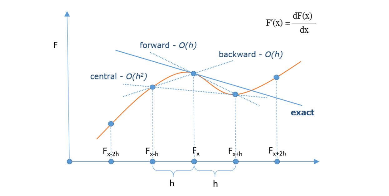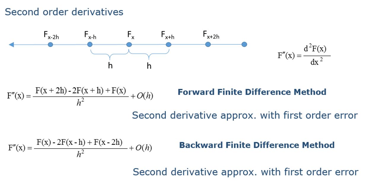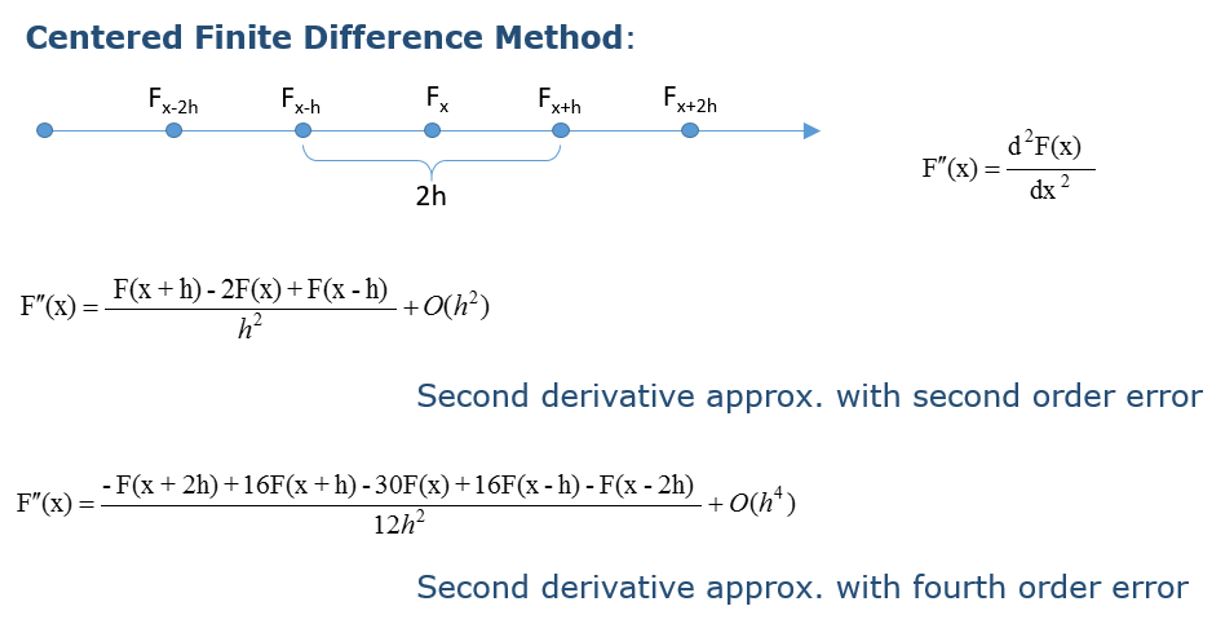
 |

Posted on:
2 Sep 2017
|
A bit more than one year back the company OTS BV came up with an innovative solution to involve Field Operators in Operator Training programs. If you haven’t read about this before or to refresh your memory, please read our previous blog post, or our white paper on this subject and also have a look at a short (2 min) movie clip in which this feature is explained.
After discussions with several interested companies a new, very interesting “spin-off” idea grew, which turns out to be very valuable for many companies that have a lot of hand valves (and/or hand operations) in the field.
Ideally, in terms of safety and good operation, every valve in a plant or tank terminal should have a position indication that is available in the Control Room. Due to obvious decisions and a balance between risk and costs it is, however, common practice that only very few hand valves have an actual position notifier.
The costs when making operation mistakes, due to wrong valve positions (resulting in contamination, spills, production loss, etc.) can be very high. Our “Smart Tag Technology” turned out to be a highly effective and low cost(!) solution to minimize operational risks, by having an overview of the actual valve positions of all (important) hand valves.
Since our Smart Tag Technology has already been implemented and used for Operator Training Scenarios (and connected to DCS systems of major vendors), the system can readily be ported to the new functionality.
In short: A field operator “scans” the position of a hand valve in the field and, without any delay, the position of this valve is visible on either the DCS or our “Dynamic P&ID Overview” computer system.
How it works
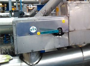
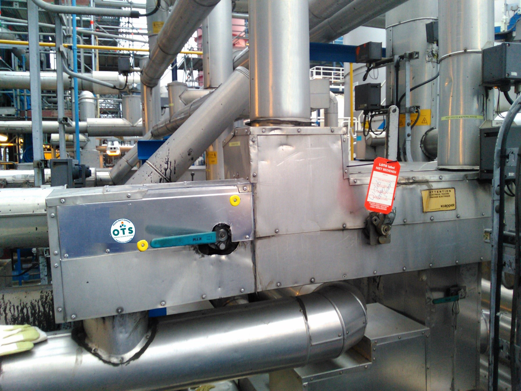
ATEX NFC Tags are mounted near hand valves.
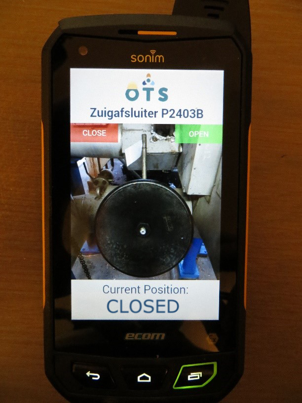
 A Tag can be scanned by an ATEX Device (which has the OTS Field App installed), after which the corresponding valve status automatically becomes visible in the control room. The communication between the ATEX device in the field and the software in the control room is done via a (very) secure and dedicated connection.
 Passing a valve position can be done in several ways. Obviously, it’s up to the end-user to choose which way(s) fits best with their business. Some options we’ve come up with so far, are:
 It’s also possible to pass a desired valve position or a list of desired valve positions (e.g. initiated from the control room) to the ATEX Device. So, after scanning an NFC Tag the actual valve position can be compared to the desired valve position and appropriate action can be taken.
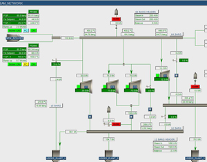
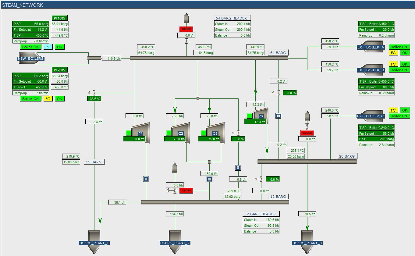
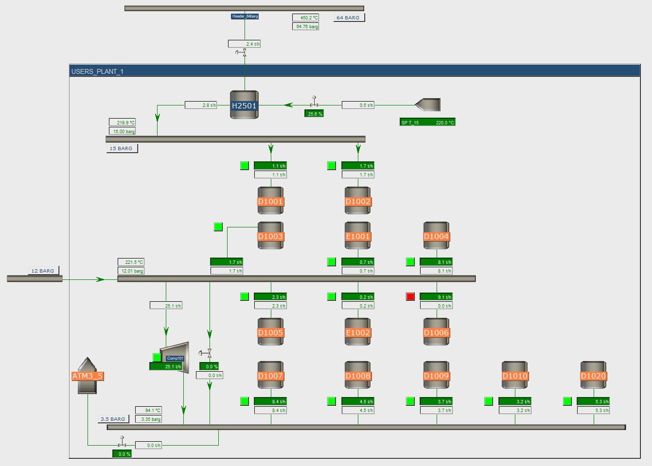
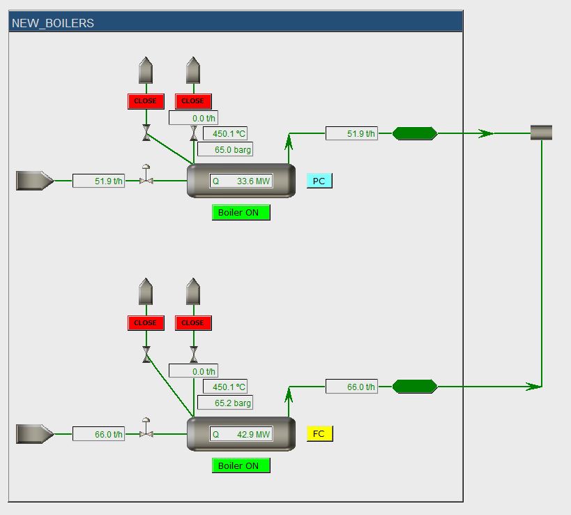
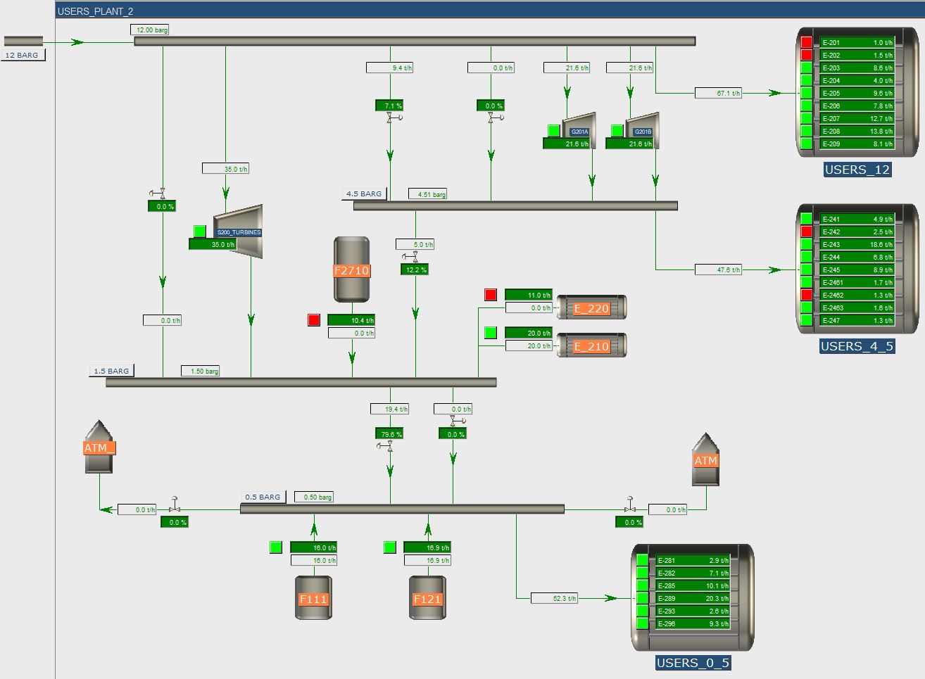
The control room has a dynamic overview showing the current valve positions. There are several possibilities for the visualization of the valve positions. Below is an example of a tank terminal, in which the open valves are colored green. The lines in which these open valves are located have a thicker line-weight to indicate that flow is possible. The closed valves in this example are white and the lines are thin.
It’s also possible to pass a desired valve position or a list of desired valve positions (e.g. initiated from the control room) to the ATEX Device. So, after scanning an NFC Tag the actual valve position can be compared to the desired valve position and appropriate action can be taken.
The control room has a dynamic overview showing the current valve positions. There are several possibilities for the visualization of the valve positions. Below is an example of a tank terminal, in which the open valves are colored green. The lines in which these open valves are located have a thicker line-weight to indicate that flow is possible. The closed valves in this example are white and the lines are thin.
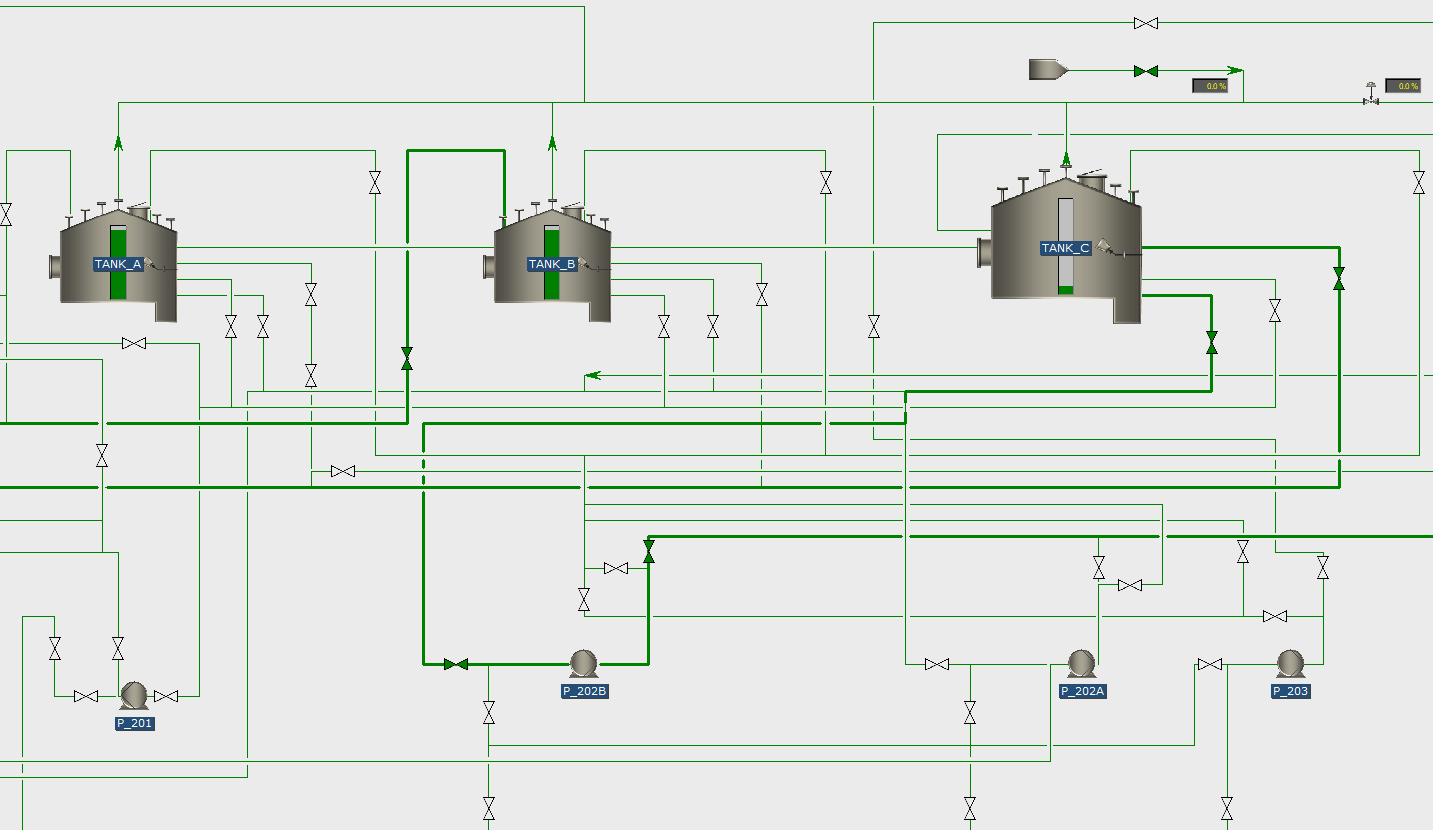 Typically, the P&ID’s are used for the dynamic valve position overviews, but optionally also the DCS screens can be adapted (and connected to the valve position software) to show the valve positions of important valves (and/or to pass desired valve positions to the ATEX Device).
In our dynamic valve position overview software you can intuitively browse through all the relevant P&ID’s. Also, the Valve Identifiers (e.g. the P&ID Tag names) can be easily shown or hidden in the overviews.
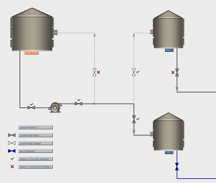
For each valve, a history list is available when it has been scanned and what the position was at that time.
If the Field App is being used for trainings, or for certain pre-defined line-ups, which involve a list of valves that need to be checked, the dynamic overview software can display whether a valve has been scanned yet and whether the valve is in the correct position (v) or not (x).
When the Tags are in place, they can be used for multiple purposes:
Typically, the P&ID’s are used for the dynamic valve position overviews, but optionally also the DCS screens can be adapted (and connected to the valve position software) to show the valve positions of important valves (and/or to pass desired valve positions to the ATEX Device).
In our dynamic valve position overview software you can intuitively browse through all the relevant P&ID’s. Also, the Valve Identifiers (e.g. the P&ID Tag names) can be easily shown or hidden in the overviews.
For each valve, a history list is available when it has been scanned and what the position was at that time.
If the Field App is being used for trainings, or for certain pre-defined line-ups, which involve a list of valves that need to be checked, the dynamic overview software can display whether a valve has been scanned yet and whether the valve is in the correct position (v) or not (x).
When the Tags are in place, they can be used for multiple purposes:
 Are you looking for a robust and affordable solution for monitoring the hand valve positions in your plant or tank terminal?
Are you looking for an effective way to train Control Room Operators and Field Operators of your plant?
Please contact us fieldapp@mobatec.nl or fieldapp@ots.expert or leave a comment in the comment box below !
To your success!
Mathieu.
———————————————–
Are you looking for a robust and affordable solution for monitoring the hand valve positions in your plant or tank terminal?
Are you looking for an effective way to train Control Room Operators and Field Operators of your plant?
Please contact us fieldapp@mobatec.nl or fieldapp@ots.expert or leave a comment in the comment box below !
To your success!
Mathieu.
———————————————–
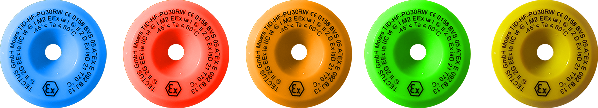
Different embodiments of ATEX NFC Tags
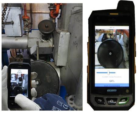
ATEX Device for scanning the Tags
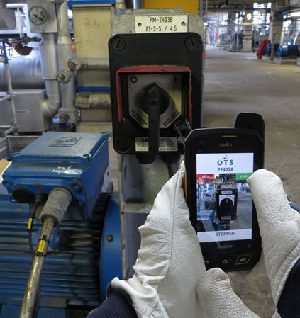
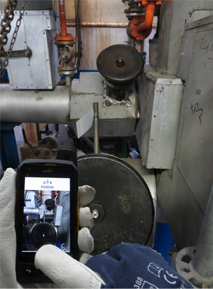
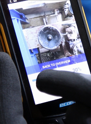
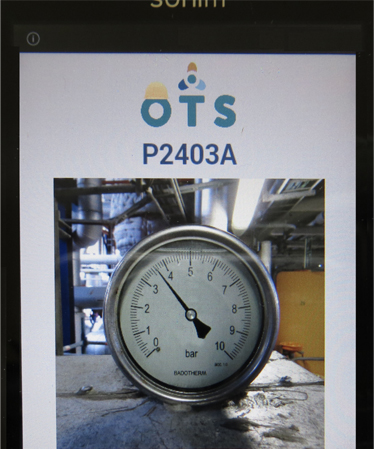
- After scanning a Tag, an “Open” and “Close” button appear with either a photo of the newly scanned valve, or an icon.
- A slider appears so that the (approximate) position (between 0 – 100%) can be communicated.
- There are two Tags mounted near the valve (e.g. a green for Open and a Red for Close), so the operator does not need to do any additional work on the ATEX Device.
- An overview of several valves appears. By clicking on one of the valves, the position of this valve can be communicated.
- More options are possible and conceivable.
Hand Valve with 2 TAGs. One for the “confirmed open” position and one for “confirmed closed”
Some more examples of possible interfaces on the ATEX Device.
Some more examples of possible interfaces on the ATEX Device.
- Hand Valve Position Overview for all kinds of purposes during normal operation
- Field Operator training for lining up certain routes.
- Operator crew trainings. So, control room operators together with field operators, training all kind of scenarios with an Operator Training Simulator.
Example of a dynamic overview for a training.