 |
 |
Apart from large scale dynamic simulation models for Operator Training Simulators, we also regularly do smaller projects and interesting case studies. In this blog post I will discuss the use of a dynamic simulation model during the design phase of a steam boiler project of one of our customers. They were interested in how their new boilers would behave dynamically and how their existing control structure would be affected by these new boilers.
With the aid of our dynamic simulation tool, they managed to successfully make some necessary changes to both their equipment and their control system, before the boilers were in service.
Process Description and Project Goal
(Note: All equipment tag names and process values have been edited on purpose, for confidentiality reasons)
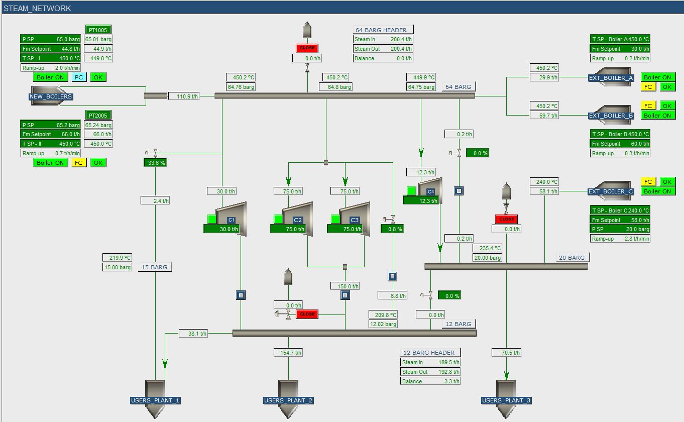
A Chemical Company invested in two steam boilers, which should provide steam to a 64 barg steam header and a connected steam network (including 20, 15, 12 barg headers and several lower pressure headers). The network is also kept on pressure by external suppliers.
 Before the company invested in the new boilers, the steam network was pressurized by the steam of a large 75 barg network of an external supplier (via a pipeline of several kilometers). The new setup would decrease the capacity (smaller holdup because of shorter distances) and therefore the company was interested in the dynamic behavior of the various steam headers in case of failure of one of the steam suppliers or other non-nominal behavior (e.g. trips in parts of the connected plants). Based on findings, the planned rules could then be adjusted.
Process Modelling
Using the supplied documents (PFD’s, P&ID’s, equipment details, etc.) and consultation with company process engineers, Mobatec set up a dynamic model, tested and tuned for the steam network. After the model was delivered, the company could perform a lot of different scenarios with the model.
The model consisted of the following components:
Before the company invested in the new boilers, the steam network was pressurized by the steam of a large 75 barg network of an external supplier (via a pipeline of several kilometers). The new setup would decrease the capacity (smaller holdup because of shorter distances) and therefore the company was interested in the dynamic behavior of the various steam headers in case of failure of one of the steam suppliers or other non-nominal behavior (e.g. trips in parts of the connected plants). Based on findings, the planned rules could then be adjusted.
Process Modelling
Using the supplied documents (PFD’s, P&ID’s, equipment details, etc.) and consultation with company process engineers, Mobatec set up a dynamic model, tested and tuned for the steam network. After the model was delivered, the company could perform a lot of different scenarios with the model.
The model consisted of the following components:
 Results
The company engineers thought of a lot of different possible scenarios and it was easy for them to implement and run these and plot and discuss relevant results.
As expected, the dynamic model confirmed that the steam headers reacted a lot quicker to offsets and disturbances with the new boiler setup as compared to previous setup (with the external supplier of 75 barg steam).
Results
The company engineers thought of a lot of different possible scenarios and it was easy for them to implement and run these and plot and discuss relevant results.
As expected, the dynamic model confirmed that the steam headers reacted a lot quicker to offsets and disturbances with the new boiler setup as compared to previous setup (with the external supplier of 75 barg steam).
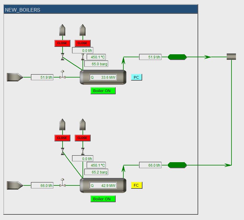 The new boiler setup was designed to operate at roughly 50% of its capacity, such that the boilers could ramp-up (or down) in case of a disturbance (like the failure of an external boiler). It was found that for most disturbances the new design and the proposed control system were just ok and the pressures in the headers would not drop below critical values, such that no (parts of) plants should be shut down.
An important change had to be implemented in the field, though, to make sure that certain plant parts would not trip after a disturbance in the steam network. The model predicted that the current size of a main “let down valve” between the 20 barg and 12 barg header was too small to cope with dynamic changes, causing one header to blow off steam, while the other dropped in pressure. Therefore, the actual valve was replaced before the new boilers where in place.
The new boiler setup was designed to operate at roughly 50% of its capacity, such that the boilers could ramp-up (or down) in case of a disturbance (like the failure of an external boiler). It was found that for most disturbances the new design and the proposed control system were just ok and the pressures in the headers would not drop below critical values, such that no (parts of) plants should be shut down.
An important change had to be implemented in the field, though, to make sure that certain plant parts would not trip after a disturbance in the steam network. The model predicted that the current size of a main “let down valve” between the 20 barg and 12 barg header was too small to cope with dynamic changes, causing one header to blow off steam, while the other dropped in pressure. Therefore, the actual valve was replaced before the new boilers where in place.
 All in all, it was a very nice project, with very positive results for the involved companies. Our customer gained better insight in the dynamic behavior of their steam network and we used the feedback of them to further improve our tools.
Let us know what you think about using dynamic simulation for industrial cases in the comment box below, such that we can all learn something from it.
To your success!
Mathieu.
———————————————–
All in all, it was a very nice project, with very positive results for the involved companies. Our customer gained better insight in the dynamic behavior of their steam network and we used the feedback of them to further improve our tools.
Let us know what you think about using dynamic simulation for industrial cases in the comment box below, such that we can all learn something from it.
To your success!
Mathieu.
———————————————–
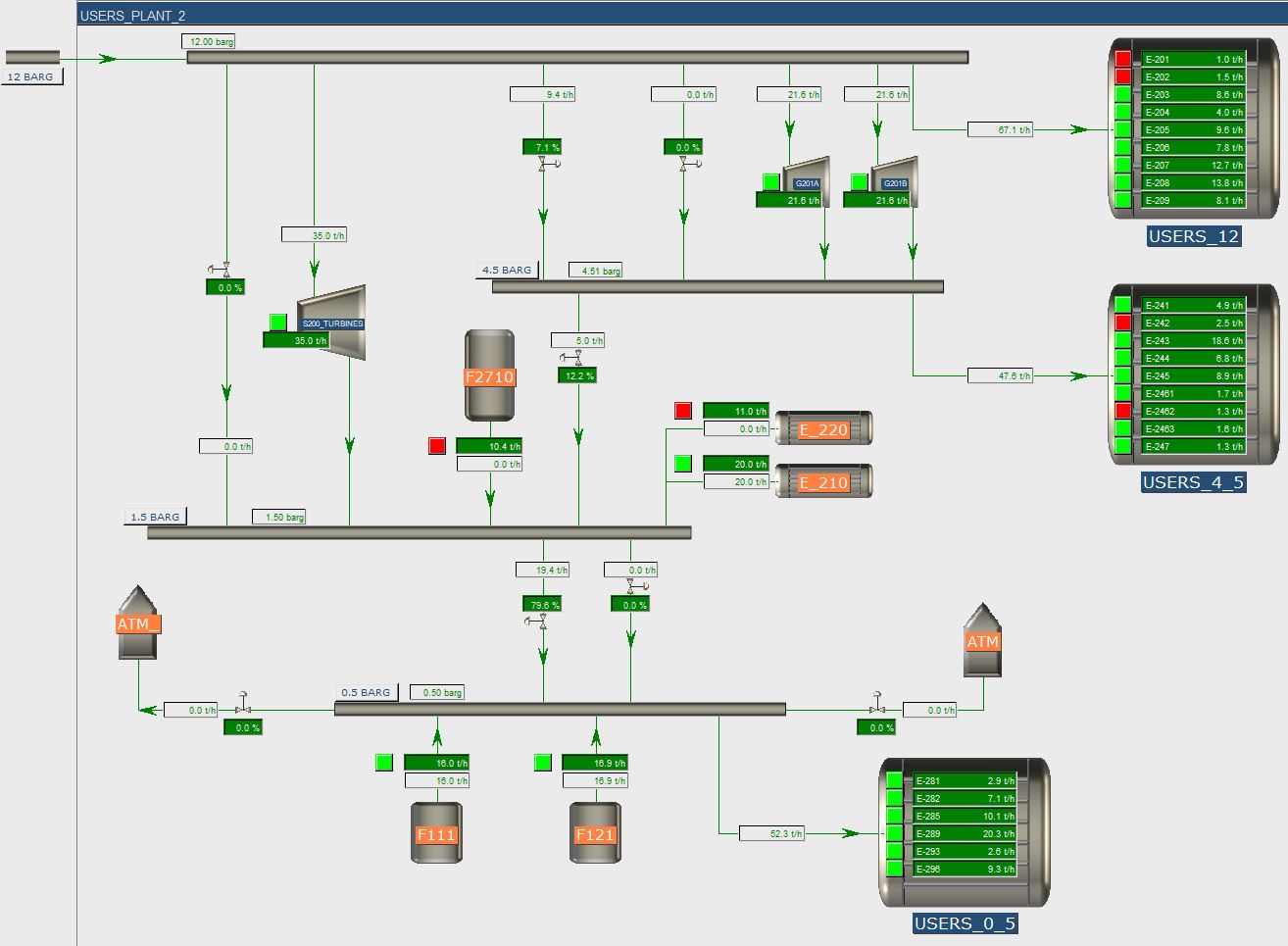
- Simplified models of all boilers, based on the boiler volume and the heat input to generate steam.
- The steam network with the main steam headers and the important control valves and controls.
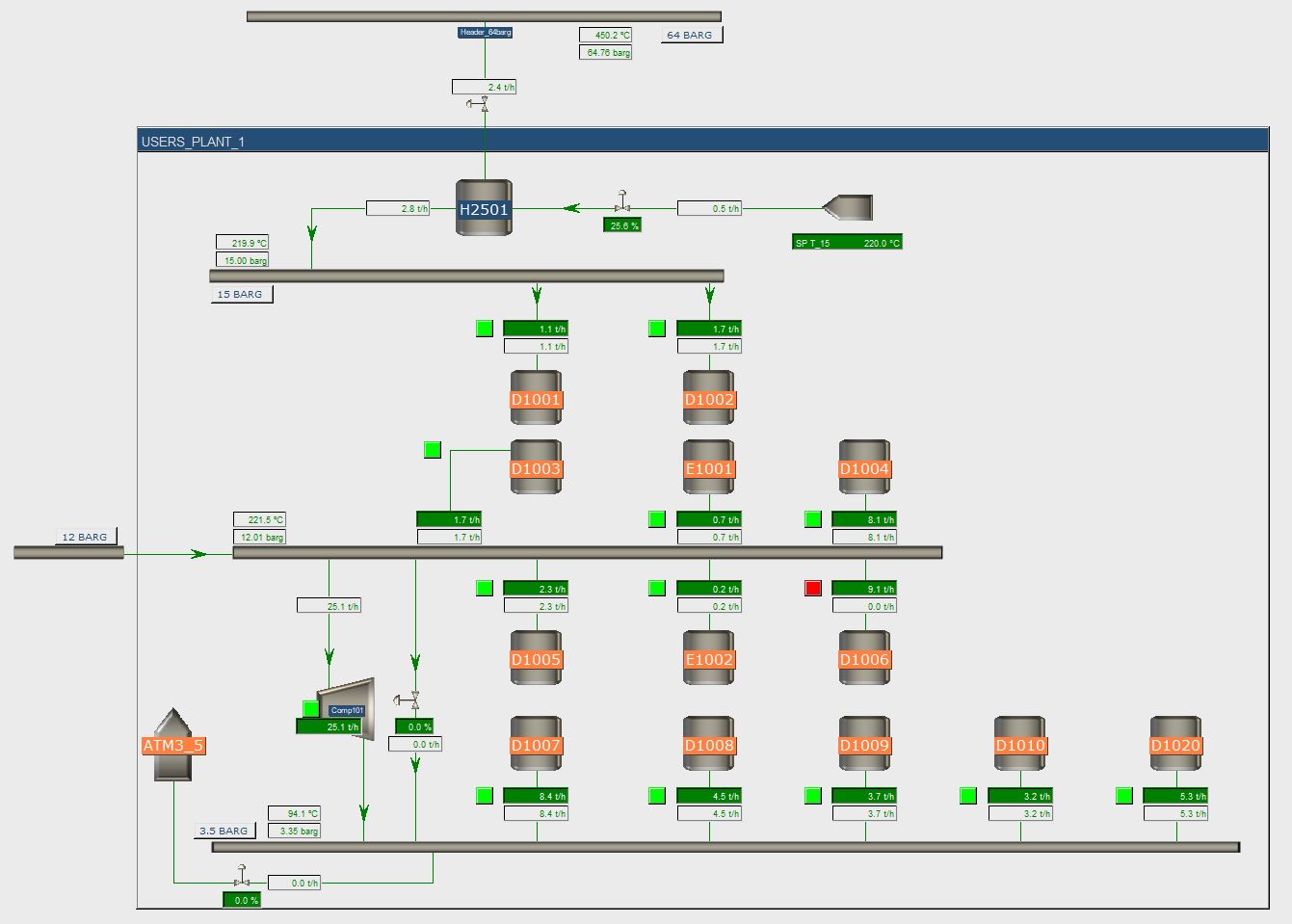
- The main customers of steam headers were modeled as “tunable customers”, such that they show realistic steam consumption under different conditions.
- All controllers, control loops and logics of interest were included in the model.