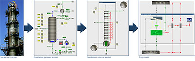
Modelling methodology implemented in Mobatec Modeller is based on the hierarchical decomposition of processes (in which material and energy exchange are playing a predominant role during normal operation) into networks of elementary systems and physical connections. The construction of a process model with this methodology consists of the following steps.
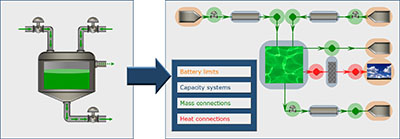
Step 1: Physical Topology
Break the process down into elementary systems that exchange extensive quantities through physical connections. The resulting network represents the physical topology.
The process of breaking the plant down to basic systems and connections determines largely the level of detail included in the model. It is consequently also one of the main factors for determining the accuracy of the description the model provides.
The process of breaking the plant down to basic systems and connections determines largely the level of detail included in the model. It is consequently also one of the main factors for determining the accuracy of the description the model provides.
Step 2: Species Topology
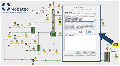
Describe the distribution of all involved chemical and/or biological species as well as all reactions in the various parts of the process.This represents the species topology, which is superimposed on the physical topology and defines which species and what reactions are present in each part of the physical topology.The species distribution is fully automated by Mobatec Modeller and is initiated by introducing species at the battery limits of the modelled process.
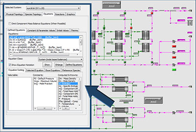
Step 3: Equation Topology
For each elementary system and each fundamental extensive quantity (component mass and energy) that characterises the system write the corresponding balance equation. Mobatec Modeller automatically generates all the needed balance equations for component mass and enthalpy of each system, since these balances can be trivially formed from the model designers definition of the physical and species topology of the process. The user cannot edit the generated balance equations!
Add algebraic equations (the so-called Constitutive Relations) to the model definition, such as transfer laws, kinetic rate expression, geometric relations, state variable transformations, etc. The dynamic balance equations and the algebraic equations, which are placed on top of the physical topology and species topology, represent the equation topology.
Add algebraic equations (the so-called Constitutive Relations) to the model definition, such as transfer laws, kinetic rate expression, geometric relations, state variable transformations, etc. The dynamic balance equations and the algebraic equations, which are placed on top of the physical topology and species topology, represent the equation topology.
Step 4: Control Scheme
Add the (dynamic) behaviour of the information processing units, such as transmitters, adjusters and controllers.
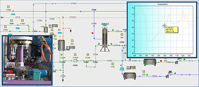
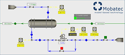
Step 5: Dynamic Simulation Run
Perform a simulation run: interact with the model, plot any variable, export data, etc.