
|

Posted on:
28 Jun 2013
|
“Process modelling is one of the key activities in process systems engineering… In most books on this subject there is a lack of a consistent modelling approach applicable to process systems engineering as well as a recognition that modelling is not just about producing a set of equations. There is far more to process modelling than writing equations”. These are a few lines from the introduction of the book “Process Modelling and Model Analysis” of Katalin Hangos and Ian Cameron. It is one of the best books around on the subject and it gives a comprehensive treatment of process modelling useful to students, researchers and industrial practitioners.
I couldn’t agree more with the statement that modelling is far more than just writing equations; the modelling activity should not be considered separately but as an integrated part of a problem solving activity. But, as promised in the previous blog, I would like to spend some lines on setting up equations for your process model.
Before we start, it is good to repeat that modelling a chemical process requires the use of all the basic principles of chemical engineering science, such as thermodynamics, kinetics, transport phenomena, etc. It should therefore be approached with care and thoughtfulness.
A (mathematical) model of a process is usually a system of mathematical equations, whose solutions reflect certain quantitative aspects (dynamic or static behaviour) of the process to be modelled. The development of such a mathematical process model is initiated by mapping a process into a mathematical object. The main objective of a mathematical model is to describe some behavioural aspects of the process under investigation.
There are many ways to generate these equations and there are many different ways to describe the same process, which will usually result in different models. The approach a modeller takes when constructing a model for a process depends on:
Having completed the first two stages of the modelling process, it is quite trivial to construct the dynamic part of the process model, namely the (component) mass and energy balances for all the systems, using the conservation principles. The resulting (differential) equations consist of flow rates and production rates, which should not be further specified at this point.
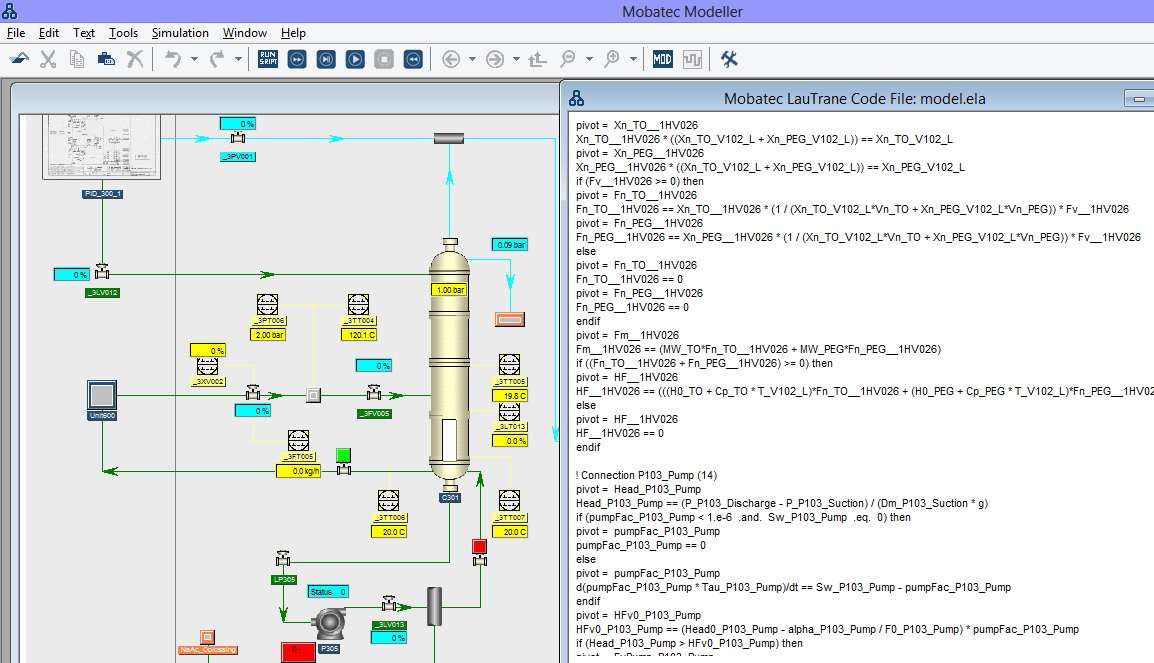
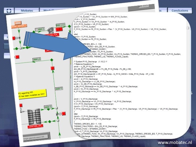
In order to fully describe the behaviour of the process, all the necessary remaining information (i.e. the mechanistic details) has to be added to the symbolic model of the process. So, in addition to the balance equations, other relationships (i.e. algebraic equations) are needed to express transport rates for mass, heat and momentum, reaction rates, thermodynamic equilibrium, and so on. The resulting set of differential and algebraic equations (DAEs) is called the equation topology.
From a certain point of view the modelling process can thus be regarded as a succession of equation-picking and equation-manipulation operations. The modeller has, virtually at least, a knowledge base containing parameterized equations that may be chosen at certain stages in the modelling process, appropriately actualized and included in the model. The knowledge base is, in most cases, simply the physical knowledge of the modeller, or might be a reflection of some of his beliefs about the behaviour of the physical process.
The equation topology forms a very important part of the modelling process, for with the information of this topology the complete model of the process is generated. The objective of the equation topology is the generation of a mathematically consistent representation of the process under the view of the model designer (who mainly judges the relative dynamics of the various parts, thus fixes intrinsically the dynamic window to which the model applies)
I couldn’t agree more with the statement that modelling is far more than just writing equations; the modelling activity should not be considered separately but as an integrated part of a problem solving activity. But, as promised in the previous blog, I would like to spend some lines on setting up equations for your process model.
Before we start, it is good to repeat that modelling a chemical process requires the use of all the basic principles of chemical engineering science, such as thermodynamics, kinetics, transport phenomena, etc. It should therefore be approached with care and thoughtfulness.
A (mathematical) model of a process is usually a system of mathematical equations, whose solutions reflect certain quantitative aspects (dynamic or static behaviour) of the process to be modelled. The development of such a mathematical process model is initiated by mapping a process into a mathematical object. The main objective of a mathematical model is to describe some behavioural aspects of the process under investigation.
There are many ways to generate these equations and there are many different ways to describe the same process, which will usually result in different models. The approach a modeller takes when constructing a model for a process depends on:
- The application for which the model is to be used. Different models are used for different purposes. For example, a model which is used for the control of a process shall be different from a model which is used for the design or analysis of that same process
- The amount of accuracy that has to be employed. This is of course partially depending on the application of the model and on the time-scale in which the process has to be modelled. In general, a model which needs to describe a process on a small time-scale demands more details and accuracy then the model of the same process which describes the process over a larger time-scale;
- The view and knowledge of the modeller on the process. Different people have different backgrounds and different knowledge and will therefore often approach the same problem in different ways, which can eventually lead to different models of the same process.
Having completed the first two stages of the modelling process, it is quite trivial to construct the dynamic part of the process model, namely the (component) mass and energy balances for all the systems, using the conservation principles. The resulting (differential) equations consist of flow rates and production rates, which should not be further specified at this point.
In order to fully describe the behaviour of the process, all the necessary remaining information (i.e. the mechanistic details) has to be added to the symbolic model of the process. So, in addition to the balance equations, other relationships (i.e. algebraic equations) are needed to express transport rates for mass, heat and momentum, reaction rates, thermodynamic equilibrium, and so on. The resulting set of differential and algebraic equations (DAEs) is called the equation topology.
From a certain point of view the modelling process can thus be regarded as a succession of equation-picking and equation-manipulation operations. The modeller has, virtually at least, a knowledge base containing parameterized equations that may be chosen at certain stages in the modelling process, appropriately actualized and included in the model. The knowledge base is, in most cases, simply the physical knowledge of the modeller, or might be a reflection of some of his beliefs about the behaviour of the physical process.
The equation topology forms a very important part of the modelling process, for with the information of this topology the complete model of the process is generated. The objective of the equation topology is the generation of a mathematically consistent representation of the process under the view of the model designer (who mainly judges the relative dynamics of the various parts, thus fixes intrinsically the dynamic window to which the model applies)
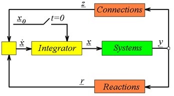
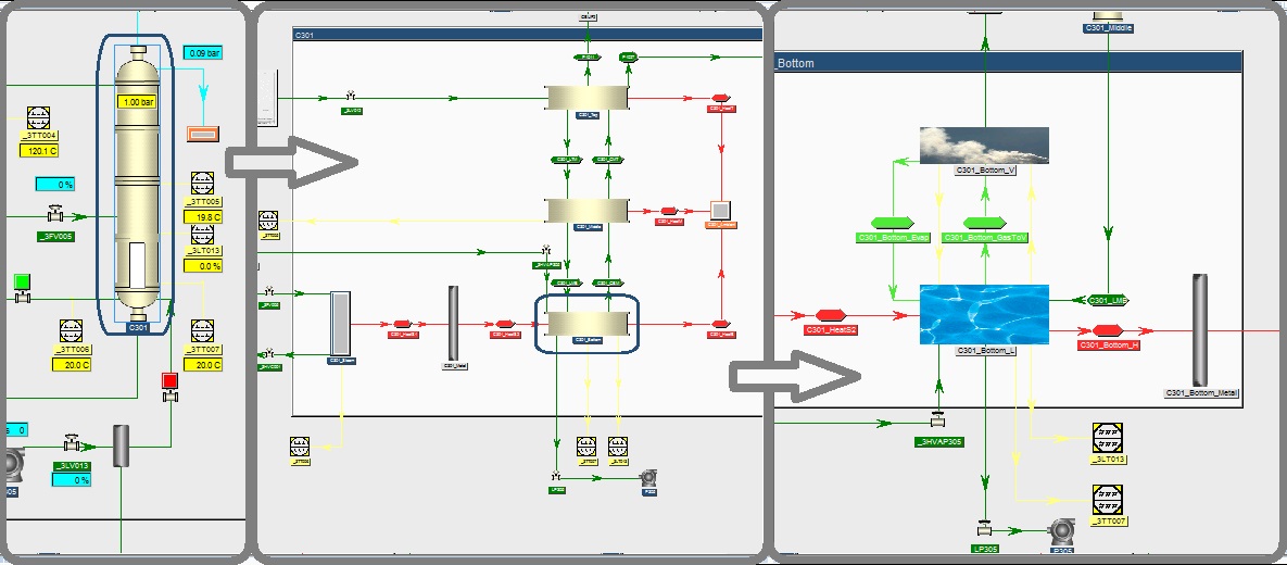
I realise that I’m just scratching the surface here, but a thorough discussion would be quite lengthy and probably just for a small audience. In the next blog I will, however, go into detail a bit more and will try to convey to you that once you understand the picture just above this text, you actually understand how any dynamic process model should be setup in order to be structurally solvable.
For now it will remain a bit abstract, but it gives you something to think about in the coming weeks :).
If you think you know what the picture represents, let everybody know by placing a comment in the comment box below. Any other comments, suggestions or questions regarding the topic of this blog would, of course, also be greatly appreciated.
To your success! Mathieu.
———————————————–